Survey Methods and Reliability Statement for Occupational Employment and Wages in Green Goods and Services

1. Introduction
2. Green Jobs Definition
3. GGS-OCC Scope
4. GGS Sample Design
5. OES Sample Design
6. Coordination Between the GGS and OES Surveys
7. Data Collection
8. Estimation Methods

I. Introduction

The Occupational Employment and Wages in Green Goods and Services (GGS-OCC) program provides data on establishments that obtain some, none, or all of their revenue from the sale of green goods and services. The estimates are based on data collected from two different Bureau of Labor Statistics (BLS) surveys: the Green Goods and Services (GGS) survey and the Occupational Employment Statistics (OES) survey, including supplemental units to the OES sample.

The GGS survey asks selected establishments how much of their revenue comes from the sale of green goods and services. The OES survey collects occupational employment and wage data for nonfarm establishments. By coordinating the GGS and OES sample designs, occupational data are collected for the majority of establishments selected into the GGS sample. A supplement to the OES survey collects data on agricultural establishments, government establishments, and additional units necessary to fully cover the scope of the GGS survey. By using data from both surveys, BLS produces occupational employment and wage estimates for businesses with all green revenue, businesses with some green revenue, and businesses with no green revenue.

II. Green Jobs Definition

BLS uses two approaches to measuring green jobs. The output approach focuses on jobs associated with producing green goods and providing green services, and the process approach focuses on jobs in which workers use environmentally friendly production processes and practices. The GGS and GGS-OCC data are based on the output approach to measuring green jobs. Green jobs estimates from the GGS survey are available on the GGS homepage. A separate survey, the Green Technologies and Practices (GTP) survey, is based on the process approach to measuring green jobs.

Under the BLS output approach, green jobs are jobs in businesses that produce goods and/or provide services that benefit the environment or conserve natural resources. These goods and services are sold to customers, and include research and development, installation, and maintenance services. Green goods and services fall into one or more of five groups:

1. Energy from renewable sources. Electricity, heat, or fuel generated from renewable sources. These energy sources include wind, biomass, geothermal, solar, ocean, hydropower, and landfill gas and municipal solid waste.
2. Energy efficiency. Products and services that improve energy efficiency. Included in this group are energy-efficient equipment, appliances, buildings, and vehicles, as well as products and services that improve the energy efficiency of buildings and the efficiency of energy storage and distribution, such as Smart Grid technologies.
3. Pollution reduction and removal, greenhouse gas reduction, and recycling and reuse. These are products and services that:
   • Reduce or eliminate the creation or release of pollutants or toxic compounds, or remove pollutants or hazardous waste from the environment.
   • Reduce greenhouse gas emissions through methods other than renewable energy generation and energy efficiency, such as electricity generated from nuclear sources.
   • Reduce or eliminate the creation of waste materials; collect, reuse, remanufacture, recycle, or compost waste materials or wastewater.
4. Natural resources conservation. Products and services that conserve natural resources. Included in this group are products and services related to organic agriculture and sustainable forestry; land management; soil, water, or wildlife conservation; and stormwater management.
5. Environmental compliance, education and training, and public awareness. These are products and services that:
   • Enforce environmental regulations.
   • Provide education and training related to green technologies and practices.
   • Increase public awareness of environmental issues.

For more information about the BLS green jobs definition, please visit the BLS green homepage.

III. GGS-OCC Scope

The scope of the GGS-OCC estimates is limited to a subset of industries in which business establishments potentially produce green goods or provide green services as their primary activity. This subset consists of 333 of the nearly 1,200 detailed industries defined by the 2007 North American Industry Classification System (NAICS). In the second quarter of 2011, these industries covered about 26 million jobs, or approximately 2.1 million establishments. These 333 industries were selected by BLS after consultations with industry groups, government agencies, stakeholders, and the public, who helped identify industries that may provide goods or services that benefit the environment or conserve natural resources. The list of in-scope industries can be found in the GGS FAQ #3. The GGS-OCC scope includes private and government establishments in the 50 states and the District of Columbia.

Businesses and government establishments are assigned industry codes based on their primary activity. Some establishments may produce green goods or provide green services as a secondary activity. BLS recognizes that if these establishments are classified in industries outside the scope of the GGS-OCC data, these goods and services and jobs associated with them will not be captured by the output approach.

IV. Description of the GGS Sample Design

The GGS-OCC sample is a subset of units in both the GGS sample and either the regular OES sample or the OES supplement. There are four major steps in obtaining the sample for GGS-OCC: (1) Use the OES sample that has already been selected, (2) select the GGS sample, (3) maximize the overlap between the OES and GGS samples, and (4) supplement the OES sample with units in GGS but not in OES. The GGS sample is a sample of 120,000 establishments in the 333 in-scope industries and was designed, in part, to maximize the overlap between it and the regular OES sample. The OES sample is a sample of 1.2 million nonfarm establishments, collected over 3 years. The OES supplement is a subsample of the GGS sample in strata where additional overlap was necessary. Below is a description of the GGS sample, the OES sample design, the OES supplement, and efforts to coordinate both surveys. For more information on GGS methodology, please see the GGS technical note. For more information on OES methodology, please see the OES technical note.

GGS Sample

The GGS sample design ensures a minimum reliability for the two main estimation domains: state by major industry sector and national by detailed industry. The GGS survey uses NAICS classifications for industry definitions.

GGS Frame Creation

The GGS sampling frame is a subset of all business establishments in the 50 states and the District of Columbia. Only establishments found in the 333 in-scope GGS industries are included on the frame. These industries were identified as the most likely to have establishments producing environmentally friendly goods or services. Private and government (federal, state, and local) establishments are included on the frame, excluding any establishment with zero employment for the past 12 months.

The GGS survey uses the BLS Quarterly Census of Employment and Wages (QCEW) as its sampling frame. The data for the QCEW come from state unemployment insurance files that are collected by individual state agencies. These files are made up of several descriptive variables such as business name, address, monthly employment, and industry classification for nearly all establishments in the United States. The 2010 QCEW has over 8 million business establishments containing about 128 million employees. The GGS sample frame, which is restricted to the 333 in-scope industries, has approximately 1.8 million establishments containing about 25.5 million employees.

About 13,000 in-scope establishments comprising about one million employees were previously identified as being involved with some kind of green activity. These units were identified internally by BLS by use of the internet and an environmental database maintained by Environmental Business International, an environmental publishing, research, and consulting company. In this statement, these 13,000 establishments will be referred to as the environmental establishment frame. These establishments have special treatment during the GGS allocation and selection phases.

The frame excludes U.S. Census Bureau establishments consisting of temporary workers hired for the 2010 decennial census.

GGS Sample Allocation

The GGS sample size was about 120,000 establishments, where 116,000 establishments were selected in a second quarter initial sample and 4,000 were selected in a fourth quarter birth sample. The initial sample was divided in the following way:

Table 1: GGS Allocation Breakout

Type of Frame Unit	Sample Allocated
Private Establishments	94,500
Local Government Establishments	7,700
State Government Establishments	4,000
Federal Government Establishments	3,300
Environmental Establishments	6,500
Total	116,000

Each type of frame unit has its own independent allocation, described below.

The GGS private establishment allocation

The GGS private establishment allocation can be thought of as two separate allocations, one that stratifies the frame by state / 2-digit NAICS industries and the other that stratifies by 4- or 6-digit NAICS industries. These 4- or 6-digit industries will be called GGS allocation NAICS, or GGS ANAICS, for the remainder of this statement. For the most part, the GGS ANAICS industries are at the 4-digit NAICS level of detail; however, some industries that seemed to be highly environmental—for example, 221119 Other Electric Power Generation—were allocated at the 6-digit NAICS level.

If the number of units in a state / 2-digit NAICS industry does not meet some threshold, all the units from the stratum are used in the GGS private sample. Otherwise, a minimum allocation is used. This allocated about 24,000 sample units for the initial 2011 sample. Next, 1,000 sample units are allocated within each state using a power allocation:

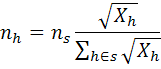
(1)

Where,

n_h = the amount of sample allocated to stratum h (state by 2-digit NAICS)

n_s = the sample size for state s, which is 1,000

X_h = the number of employees in stratum h

After the minimum and power allocation, a total of about 60,000 sample units were allocated for private establishments in 2011. Thus, a sample of 60,000 ensures a minimum sample of 1,000 establishments per state and 40 establishments for each 2-digit NAICS within a state.

Next, the sample is allocated nationally to GGS A_NAICS industry strata, using the following power allocation:

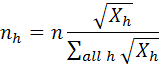
(2)

Where,

n_h = the amount of sample allocated to stratum h (GGS A_NAICS)

n = the national sample size

X_h = the number of employees in stratum h

The national sample size is iteratively increased until the total private allocation, after reconciling the state by 2-digit and national GGS A_NAICS allocations, is close to 94,500. The last step of the private allocation is to set a minimum allocation to each 6-digit NAICS stratum. However, if the number of units in the 6-digit national stratum does not meet some threshold, all of the establishments in the stratum are used in the sample. In the initial 2011 sample, there were a total of about 94,800 sample units allocated for the private sample.

The local, state, and federal government GGS allocations

The sample units for local, state, and federal government establishments are allocated the same way. The frame is stratified into state and 2-digit NAICS industry strata. If the number of establishments within a stratum does not meet some threshold, all of the units from the stratum are allocated into the sample. Otherwise, a minimum allocation is used. In the initial 2011 sample, the local allocation was 7,700 units, the state allocation was 3,950 units, and the federal allocation was 3,300 units.

Environmental GGS allocation

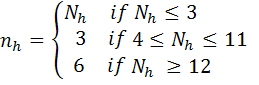
The environmental allocation includes establishments in the private and government sectors. The frame is stratified by 6-digit NAICS industry and size class. Size classes are seven categories that put establishments of similar employment size together. For example, if an establishment has 1 to 9 employees, it would be in size class 1 for GGS. The environmental sample is allocated using the following rules:

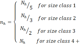
(3)

Where,

n_h = the amount of sample allocated to stratum h (6-digit NAICS by size class)

N_h = the number of frame units in stratum h

In the initial 2011 sample, there were about 6,550 sample units allocated for the environment sample.

GGS Sample Selection

The private and government samples are selected using a probability proportionate to size approach where the size for an establishment is defined below:

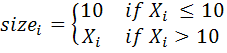
(4)

Where,

size_i = unit i 's measure of size

X_i = unit i 's maximum employment over previous 12 months

The smallest establishments are treated differently because of the assumption that they have the potential for very large relative employment shifts between the time period of the QCEW data on the frame and when the establishment is sampled.

The environmental sample is selected using simple random sampling within each national 6-digit NAICS by size class stratum. The sample is allocated at higher rates as the size class increases, resulting in an implicit probability proportionate to size selection scheme.

GGS Birth Sample

A fourth quarter birth sample of about 4,000 establishments is selected to represent the newly formed establishments that become in business or in-scope between the second quarter and the fourth quarter of 2010. Any establishment in the fourth quarter 2010 sample frame that is not in the second quarter 2010 sample frame is considered a birth. The birth sample is allocated at the same rate as the initial sample for each of the five different allocations.

Sampling Weights

Each sampled establishment has a known probability of selection. The inverse of the probability of selection is called the sampling weight.

V. Description of the OES Sample Design

The OES survey is designed to collect occupational employment and wage data on employees working in the 50 states, the District of Columbia, the Virgin Islands, Puerto Rico, and Guam. The main estimation domain is at the level of detailed Metropolitan Statistical Areas (MSA) and residual areas within each state called balance of state (BOS) areas. To produce estimates in such detail, a sample of 1.2 million business establishments is selected over 3 years in semiannual samples. A sample of 200,000 establishments is selected in the second and fourth quarter of each year.

OES Frame Creation

The OES survey also uses the QCEW as its sampling frame. The majority of NAICS industries are in scope for OES, except for NAICS 814 Private households, and most of the agriculture sector with the exception of 113310 Logging, 1151 Support activities for crop production, and 1152 Support activities for animal production. The second quarter 2011 OES frame had about 6.8 million in-scope business establishments that account for about 121 million employees.

OES Sample Allocation

The OES frame stratification is by state, MSA or BOS area, and 4-, 5-, or 6-digit NAICS industries. The majority of the strata use 4-digit NAICS detail, but some industries are stratified in more detail because they have unique occupational distributions at the 5- and 6-digit level. These 4-, 5-, or 6-digit NAICS industries will be referred to as OES allocation NAICS, or OES A_NAICS.

For each semiannual sample, a full 1.2 million establishment sample is allocated, and then the allocation is divided by six at the stratum level. First, a minimum sample is allocated using the following rules:

(5)

Where,

n_h = the amount of sample allocated to stratum h (State by MSA/BOS by OES A_NAICS)

N_h = the number of frame units in stratum h

Next, the sample is allocated using a power Neyman allocation, using the following formula:

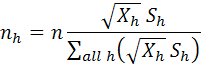
(6)

Where,

n_h = the amount of sample allocated to stratum h (State by MSA/BOS by OES A_NAICS)

n = the national sample size

X_h = the number of employees in stratum h

S_h = the measure of occupational employment variability within stratum h

The final amount of sample allocated for each stratum is the maximum of the minimum and power Neyman allocations. The national sample size used in formula (6) is iteratively changed until the final amount of sample allocated, after reconciling the two different allocations, is about 1.2 million. The last step of the OES allocation is to divide each stratum allocation amount by six, to get the final allocation for the semiannual sample.

OES Sample Selection

After the sample is allocated, the semiannual sample is selected using a probability proportionate to size approach. Every establishment within an OES-defined size class is given the average employment value for that size class. This is referred to as a step-wise probability proportionate to size scheme.

Sampling Weights

Each sampled establishment has a known probability of selection. The inverse of the probability of selection is called the sampling weight.

VI. Coordination between the GGS and OES Surveys

A 100-percent sample overlap between the GGS and OES would be the ideal situation for producing the GGS-OCC estimates because it would allow OES to survey every establishment in the GGS sample. To achieve a 100-percent sample overlap, the GGS sample would need to be selected as a subsample of the OES sample. For several reasons, including coverage bias and budget constraints, this was not a viable option. Instead, special methods are used to ensure a maximum sample overlap between the GGS and OES samples. The GGS-OCC estimates use the GGS initial and birth samples collected in the second and fourth quarters of 2011, respectively, and the OES samples collected in the second and fourth quarters of 2009, 2010, and 2011. Three years of OES sample are used based on the assumption that occupational employment distributions stay consistent over 3-year time periods. Special methods are used to age OES wage data that were collected during a time period outside of the reference period.

Natural Sample Overlap between GGS and OES

In both the GGS and OES sample designs, a greater probability of selection is given to establishments with more employees. This causes a substantial amount of overlap between the two samples, even if they have independent sample designs. In 2011, approximately 41 percent (about 41,300 sampled establishments) of the GGS initial and birth sample overlaps naturally with the OES sample collected between 2009 and 2011. The overlap is higher for large establishments, decreasing as establishments get smaller. This causes the sample employment overlap to be significantly larger than the unit overlap, at 80 percent of in-scope employment (about 8.3 million employees).

Most of the state and local government units had to be excluded from these sample overlap counts because OES and GGS define their public Primary Sampling Units (PSUs) differently. In the OES sample, state and local government PSUs are aggregated to specific geographic areas to make data collection easier for the state data collectors. In the GGS sample, state and local government PSUs are single business establishments. Only OES state and local aggregate PSUs that contain only one establishment are used when identifying the natural overlap between the two surveys and in the replacement algorithm described later.

Increasing Overlap through Replacement

To increase the overlap for the smaller establishments, an algorithm is used that replaces nonoverlapping GGS sampled units with nonoverlapping OES sampled units. All establishments from the environmental frame were excluded from this process because they were predetermined to have green activity and therefore important to keep in the GGS sample. The replacement algorithm uses strict criteria to minimize any bias this process could introduce. In order for an establishment sampled for GGS to be replaced by one from OES, it must meet the following criteria:

• Industrial criterion: The GGS and OES sampled establishments must have the same 6-digit NAICS industry classification
• Geographic criterion: The GGS and OES sampled establishments must be within the same state, first giving preference to establishments in the same state and MSA/BOS area, then relaxing the search to just state
• Age criterion: The GGS and OES sampled establishments must have begun their business in the same year and quarter if they have been in business less than 3 years

• Employment criterion: The GGS and OES sampled establishments must meet the following employment tolerances:

  
  

  GGS Employment	OES Employment
  1 to 4	1 to 4
  5 +	0.9 × GGS_Emp to 1.1 × GGS_Emp

  
  
• Multi-establishment criterion: The GGS and OES sampled establishments must both be from a company that has multiple establishments, or both from a company that has only one establishment

In 2011, after using this replacement algorithm, the amount of sample overlap between the GGS and OES surveys increased to 64 percent (about 64,700 sampled establishments). The amount of sample employment overlap increased slightly to 83 percent (about 8.6 million employees).

Subsample of the Nonoverlapping GGS Sample

To collect occupational employment and wage data for the piece of the GGS sample that does not overlap with OES, a subsample of 25,000 establishments was selected. These establishments are asked occupational information by being sent an OES survey form in addition to a GGS survey form.

The nonoverlapping GGS sample is stratified by 6-digit NAICS industries and the subsample is allocated using the following formula:

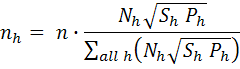
(7)

Where,

n_h = the number of subsample units allocated to industry h (6-digit NAICS)

n = the total subsample size

S_h = the measure of occupational employment variability within stratum h (6-digit NAICS)

N_h = the number of nonoverlapping GGS sample units within stratum h

P_h = the nonoverlap employment percentage for stratum h

This allocation method allows the sample size for a particular 6-digit NAICS industry to increase as the amount of nonoverlapping GGS sample and the occupational employment variability of that industry increase.

The first step of selecting the subsample is to identify the units within each 6-digit NAICS industry that will make the largest contribution to the variance estimate, and select them with certainty. The amount of the GGS universe each nonoverlapping GGS sample unit represents is calculated as:

(8)

Where,

E_i = establishment i 's weighted employment

w_i = establishment i 's GGS sampling weight

x_i = establishment i 's QCEW employment

Next, the average weighted employment is calculated for each 6-digit NAICS industry by:

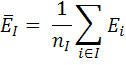
(9)

Where,

_I = the amount of weighted employment each subsample unit will represent on average

If any unit’s E_i is greater than or equal to _I, then it is selected into the subsample with certainty. This is an iterative process in which each time establishments are selected with certainty, _I is recalculated and compared to the remaining unit’s E_i. Once there are no more units to select with certainty, the remaining units are selected within each industry using simple random sampling (SRS). The final weight that will be used for the occupational estimates for the GGS sampled units selected into the subsample is the product of their original GGS weight and the inverse of their subsampling selection probability.

VII. Data Collection

OES Data Collection

The OES survey collects data on occupational employment and wage rates for wage and salary workers. Respondents report their number of employees by occupation across twelve nonoverlapping wage intervals:

Table 2: OES Wage Intervals

Interval	Wages
	Hourly	Annual
A	< $9.25	<$19,240
B	$9.25 to $11.49	$19,240 to $23,919
C	$11.50 to $14.49	$23,920 to $30,159
D	$14.50 to $18.24	$30,160 to $37,959
E	$18.25 to $22.74	$37,960 to $47,319
F	$22.75 to $28.74	$47,320 to $59,799
G	$28.75 to $35.99	$59,800 to $74,879
H	$36.00 to $45.24	$74,880 to $94,119
I	$45.25 to $56.99	$94,120 to $118,559
J	$57.00 to $71.49	$118,560 to $148,719
K	$71.50 to $89.99	$148,720 to $187,199
L	≥$90.00	≥$187,200

The OES survey form asks the respondent to report how many employees fall within each occupation by wage interval category. The respondent reports this information into a reporting matrix, where the occupations run down the rows, and the wage intervals span across the columns. The Standard Occupational Classification (SOC) system is used to define occupations. Below is an example of an OES reporting matrix for a restaurant establishment:

GGS Data Collection

The GGS survey asks establishments to report the percent of revenue received from green goods and services as defined by BLS. The percentage is multiplied by the employment level to derive the number of GGS jobs for that establishment. Units that do not generate revenue, such as nonprofits, government units, and business start ups without positive revenue, are asked to supply a percent of employment associated with green goods and services. Thus, the employment figure includes workers of all occupations, as long as they worked in the establishment with GGS employment or revenue. For example, a solar panel installation business might report that all of its revenue is included in the definition. In this case, all workers are counted, including installers, managers, secretaries, etc. Similarly, mass transit businesses reporting GGS revenue would include workers such as bus and subway drivers, maintenance and repair workers, managers, and administrative personnel.

Response Rates

Among GGS-OCC sample units, the overall national response rates for the GGS survey were 66.4 percent based on establishments and 59.9 percent based on weighted employment. Response rates for the OES survey were 66.7 percent based on establishments and 65.3 percent based on weighted employment. About 48.6 percent of sampled establishments, representing 42.6 percent of weighted sample employment, responded to both surveys.

VIII. Estimation Methods

GGS-OCC Micro Data

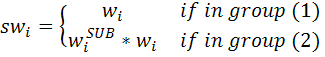
The data that are used for the GGS-OCC estimates come from establishments that were sent both OES and GGS survey forms. These establishments fall into two groups: (1) the establishments that were selected into both the GGS and OES samples, and (2) the establishments that were selected into the GGS sample but not the OES sample, and then were subsampled from the GGS to receive an OES survey form. In 2011, the sample consisted of approximately 93,200 establishments (including federal units). The sampling weight used for group (1) is the GGS sampling weight, and for group (2) is the product of the subsampling weight and the GGS sampling weight. The sampling weight for establishment i from the GGS-OCC data is:

(10)

Where,

w_i = establishment i 's GGS sampling weight

w_i^sub = establishment i 's subsampling weight

When using these sampling weights, the 93,200 GGS-OCC establishments correctly represent all in-scope establishments for the GGS universe.

Nonresponse Adjustments

Survey nonresponse occurs when units that were selected into the sample fail to provide all the information that was solicited. Sometimes the failure is partial, meaning the unit provides information for only some items in the survey. Other times the failure is complete, meaning the unit provided no information for the survey. The partial failure is referred to as item nonresponse, and the total failure as unit nonresponse. If the information collected from the respondents differs from the information that would have been collected for the nonrespondents, then there is potential for bias in the survey estimates. To reduce this nonresponse bias, imputation is often used to handle item nonresponse, and weight adjustments for unit nonresponse.

Every establishment within the GGS-OCC data can be grouped into one of four different response categories: (1) responds to both the GGS and OES survey forms, 48.6 percent of sampled units; (2) responds to the GGS survey form but does not respond to the OES survey form, 17.9 percent of sampled units; (3) does not respond to the GGS form but responds to the OES form, 15.8 percent of sampled units; and (4) does not respond to either the GGS or OES forms, 17.8 percent of sampled units. For the GGS-OCC estimates, response category (2) is considered item nonresponse and (3) and (4) are considered unit nonresponse. To reduce nonresponse bias, imputation is used to handle the GGS-OCC item nonresponse, and weighting class adjustments are used to handle the unit nonresponse.

Imputation

A nearest neighbor hot deck imputation is used to impute staffing patterns—the share of an establishment’s employment that falls into each occupation—for establishments found in response category (2). State, industry, employment, and green revenue percent are used to determine a donor for the nonrespondents. The donor will provide occupational employment distributions for the establishment with no OES data. For units that report having 0 or 100 percent green revenue, the imputation cells are defined by state/6-digit NAICS industry/green revenue percentage and the nearest neighbor donor is found based on employment (the donor will use the reported total OES employment, and the nonrespondent will use QCEW employment). For units that have green percentages greater than 0 and less than 100, the imputation cells are defined by state/6-digit NAICS and the nearest neighbor donor is found based on both green revenue percentage and employment. A hierarchical structure is used to determine how to collapse the imputation cells in case there are no or too few available donors. In this hierarchy, geographical level is the first criterion to be relaxed, because industry is the most important determinant of staffing patterns.

A mean imputation procedure is used to impute average wage distributions for establishments in response category (2). Geography, industry, employment, and green revenue percent are used to create imputation cells for imputing the missing wage distributions. Using all responding units, average wage distributions are calculated within each imputation cell. Units with missing wage data receive the average wage distribution of their imputation cell. A hierarchical structure is used for collapsing imputation cells that do not have enough respondents to make an average wage distribution. Wages are more homogeneous within geography, so in this hierarchy industry is the first characteristic to be relaxed.

Weighting class adjustments

For establishments in response categories (3) and (4), an iterative weighting class adjustment process is used to adjust the sample weights so that the respondents are representative of the entire GGS-OCC universe. This process has 3 stages: the first adjusts weights at the ownership by size class level, the second adjusts weights at the 6-digit NAICS by collapsed size class level, and the third adjusts weights at the state by 2-digit NAICS level. The weights are modified at each stage by multiplying a nonresponse adjustment factor (NRAF) by all weights within weight classes so that weighted respondent counts are calibrated to equal weighted sample counts. The raking procedure is repeated until the NRAFs for all weight classes converge to 1. A final NRAF value is calculated for each establishment by multiplying the NRAFs calculated at each stage and iteration. The final NRAF for establishment i  is denoted FNRAF_i.

Benchmarking

Due to differences between the date of sample selection and the reference period of the estimates, the GGS-OCC data are benchmarked to QCEW average employment levels for May and November 2011. Like the weighting class adjustments, the benchmarking process is an iterative process. It has two stages: the first adjusts weights at the allocation NAICS (or GGS A_NAICS) level, and the second adjusts weight at the state by 2-digit NAICS level. The weights are modified at each stage by multiplying all weights within the benchmarking classes by a benchmarking factor (BMF) so that weighted respondent counts are calibrated to equal average QCEW counts. The raking procedure is repeated until the BMFs for all benchmarking classes converge to 1. A final BMF value is calculated for each establishment by multiplying the BMFs calculated at each stage and iteration. The final BMF for establishment i  is denoted FBMF_i.

Point Estimates

The GGS-OCC data consist of employment, mean wage, and median wage estimates by occupation, presented for three groups of establishments: those with all, none, or some, but not all, of their revenue from green goods and services. Estimates are available at the national level for 2-digit NAICS industries and for all in-scope industries combined. There are three different occupational levels for the estimates: all-occupations totals, major occupational groups, and detailed occupations. These levels are defined by the Standard Occupational Classification (SOC) system. The reference period for these estimates is November of 2011.

Employment estimates

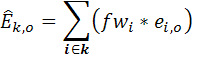
A Horvitz-Thompson (HT) estimator is used for the GGS-OCC employment estimates. The GGS-OCC employment estimate for estimation domain k  is calculated using the formula:

(11)

Where,

_k,o = the total employment estimate for occupation o, in estimation domain k

 

fw_i = the final estimation weight for establishment i , which is the product of the sampling weight, the final nonresponse adjustment factor, and the final benchmark factor:

fw_i = sw_i × FNRAF_i × FNBMF_i

e_i,o = the OES reported employment for occupation o within establishment i

Mean wage estimates

Because wages are collected in intervals rather than point values, an external file from the National Compensation Survey (NCS) is used to calculate interval means that are assigned to all employees falling within each of the 12 wage intervals. Also, because the wage data are collected over 3 years, the older data are aged by the Employment Cost Index (ECI) for different occupational groups. The ECI is produced by NCS and measures the rate of change in employee compensation over time.

Using the data collected by OES plus the information obtained from NCS, the GGS-OCC wage estimates are calculated using the following formula:

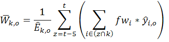
	(12)
	(13)

Where,

= the hourly wage rate estimate for occupation o, in estimation domain k

t = the current panel (2011Q4), t - 1 equals the previous panel, etc.

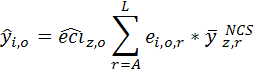
= the estimated wage for occupation o, within establishment i

= the ECI aging factor for panel z and occupation o

e_i,o,r = the reported employment for occupation o, within establishment i, within wage interval r

 

= the NCS wage interval mean for wage interval r, in panel z

To calculate GGS-OCC annual wage rate estimates, the hourly estimates are multiplied by 2,080, based on the assumption that most full-time employees are paid for 2,080 hours a year (52 weeks x 40 hours per week).

Median hourly wage rate estimates

The median or 50^th percentile hourly wage rate for an occupation is the wage where 50 percent of all workers earn that amount or less and where 50 percent of all workers earn that amount or more. The wage interval containing the median hourly wage rate is located using a cumulative frequency count of estimated employment across all wage intervals. After the targeted wage interval is identified, the median wage rate is then estimated using a linear interpolation procedure. This statistic is calculated by first uniformly distributing federal, state, local government, and private workers inside each wage interval. Next, workers are ranked from lowest paid to highest paid. The product of the total employment for the occupation and the 50^th percentile is then calculated to determine the worker that earns the median wage rate. Finally, the following formula is then used to calculate estimates of the 50^th percentile wage rate for each occupation in the predetermined estimation cell.

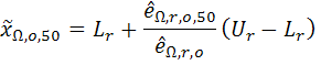
(14)

Where,

r = the universal wage interval that encompasses the 50^th percentile wage rate estimate

Ω = a predetermined estimation cell

L_r = the lower bound of universal interval r  expressed in terms of hourly wage rate

U_r = the upper bound of universal interval r  expressed in terms of hourly wage rate

_Ω,r,o = the OES reported employment in estimation cell Ω and universal interval r  for occupation o

 

_Ω,r,o,50 = the OES reported employment in estimation cell Ω and universal interval r  for occupation o needed to reach the 50^th percentile

 

_o,50 = the estimated 50^th percentile wage rate estimate for occupation o in cell Ω

Variance Estimates

When a sample, rather than an entire population, is surveyed, estimates differ from the true population values that they represent. This difference, or sampling error, occurs by chance and its variability is measured by the variance of the estimate or the standard error of the estimate (square root of the variance). The relative standard error is the ratio of the standard error to the estimate itself.

Estimates of the sampling error for the GGS-OCC employment and wage estimates allow data users to determine if those statistics are reliable enough for their needs. Only a probability-based sample can be used to calculate estimates of sampling error. The formulas used to estimate GGS-OCC variances are adaptations of formulas appropriate for the survey design used.

The particular sample used in this survey is one of a large number of many possible samples of the same size that could have been selected using the same sample design. Sample estimates from a given design are said to be unbiased when an average of the estimates from all possible samples yields the true population value. In this case, the sample estimate and its standard error can be used to construct confidence intervals, or ranges of values that include the true population value with known probabilities. To illustrate, if the process of selecting a sample from the population were repeated many times, if each sample were surveyed under essentially the same unbiased conditions, and if an estimate and a suitable estimate of its standard error were made from each sample, then:

1. Approximately 68 percent of the intervals from one standard error below to one standard error above the estimate would include the true population value. This interval is called a 68-percent confidence interval.
2. Approximately 90 percent of the intervals from 1.645 standard errors below to 1.645 standard errors above the estimate would include the true population value. This interval is called a 90-percent confidence interval.
3. Approximately 95 percent of the intervals from 1.96 standard errors below to 1.96 standard errors above the estimate would include the true population value. This interval is called the 95-percent confidence interval.
4. Almost all (99.7 percent) of the intervals from 3 standard errors below to 3 standard errors above the estimate would include the true population value.

Employment variance

To measure the variability of the GGS-OCC employment estimate, a random group jackknife replicate variance estimator is used. In this technique, each sampled establishment is assigned to one of G random groups. All establishments in each group are considered one of G different subsamples. Each subsample is reweighted to represent the universe.

G estimates of total occupational employment, _k,o,g (one estimate per subsample) are calculated. The variability among the G employment estimates is a good variance estimate for occupational employment. The two formulas below are used to estimate the variance of occupational employment for an estimation domain defined by k :

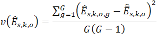
(15)

Where,

_s,k,o = the total employment estimate for occupation o, in estimation domain k, for size class s

 

_s,k,o,g = the total employment estimate for occupation o, in estimation domain k, for size class s, using subsample g

 

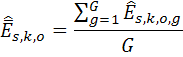
_s,k,o = the average total employment for occupation o, in estimation domain k, for size class s, across all G subsamples. Where,

The variance of the GGS-OCC employment estimate is the sum of all the variances for each size class estimate calculated in formula (16):

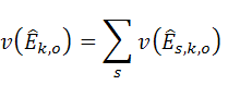
(16)

The standard error and percent relative standard error are calculated using the formulas below, respectively:

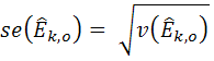
	(17)
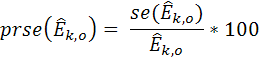
	(18)

Wage variance

To measure the variability of the GGS-OCC wage estimates, Taylor Series Linearization techniques were used to develop an estimator. Some components of the wage variance are to capture the added variability to the wage estimates caused by collecting interval data and using NCS data to give each employee a wage value. The first component of the variance formula accounts for the design-based variance. The other three components account for using intervals to collect the data. The formula below is used to estimate the variance of occupational hourly wage rate estimates for an estimation domain defined by h:

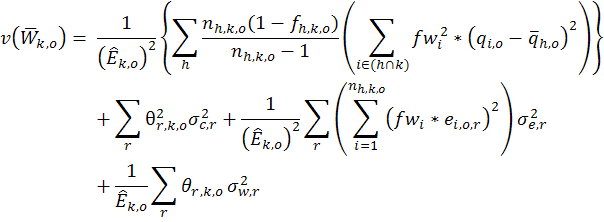
(19)

Where,

n_h,k,o = the number of sampled establishments in stratum h, and estimation domain k, that have occupation o

 

f_h,k,o = the sampling fraction in stratum h, from establishments in estimation domain k, that have occupation o

 

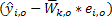
q_i,o =  for occupation o in establishment i

 

_h,o = the average q_i,o value in stratum h

 

Θ_r,k,o = the proportion of employment in wage interval r, for occupation o, within establishments in estimation domain k

 

= within wage interval r, these are estimated using the NCS and, respectively, represent the variability of the wage value imputed to each worker, the variability of wages across establishments, and the variability of wages within establishments

Confidentiality

BLS has a strict confidentiality policy that ensures that the survey sample composition, lists of reporters, and names of respondents will be kept confidential. Additionally, the policy assures respondents that published figures will not reveal the identity of any specific respondent and will not allow the data of any specific respondent to be inferred. Each published estimate is screened to make certain that it meets these confidentiality requirements. To further protect the confidentiality of the data, the specific screening criteria are not listed in this publication.

 

Last Modified Date: October 3, 2012