An official website of the United States government
An official website of the United States government
The .gov means it's official.
Federal government websites often end in .gov or .mil. Before sharing sensitive information,
make sure you're on a federal government site.
The site is secure.
The
https:// ensures that you are connecting to the official website and that any
information you provide is encrypted and transmitted securely.
In 2014, the Producer Price Index (PPI) program of the Bureau of Labor Statistics (BLS) transitioned from the Stage of Processing (SOP) system to the Final Demand–Intermediate Demand (FD–ID) system as the key structure used for analyzing the behavior of producer prices. The FD–ID system expanded PPI aggregate index coverage beyond that of the SOP system (which included only goods sold for personal consumption and as private capital investment) through the addition of indexes for services, construction, exports, and government purchases.
The FD–ID system comprises two main portions: final demand and intermediate demand. The final-demand portion of the system measures price change for goods, services, and construction products sold for personal consumption, as capital investment, for export, and to government. Final demand represents the last stage in the domestic chain of production, because final-demand products are sold to an end user and are not used as an input to another domestic product. Examples of final-demand products include automobiles sold to consumers, textile machinery sold as capital investment, legal services purchased by the government, healthcare services sold for personal consumption, and construction sold as capital investment. The intermediate-demand portion of the FD–ID system measures price change for goods, services, and construction products sold to businesses as inputs to production, excluding capital investment. Intermediate-demand products can be used as inputs to other intermediate-demand products or as inputs to final-demand products. Crude petroleum sold to refineries, car parts sold to automobile manufacturers, and business consulting services sold to accounting firms are examples of intermediate-demand products.
In order to meet the needs of different data users, the FD–ID aggregation system includes two separate treatments of intermediate demand, each designed for a different analytical use. The first treatment organizes intermediate-demand products by type of product, establishing a “commodity-type model” of price change. The intermediate-demand indexes in this model provide value to data users by supplying specific information about the type(s) of products creating inflationary pressure in the economy. The second treatment organizes the same intermediate-demand commodities1 into a production-flow model. The production-flow model assigns commodities to stages in such manner that the commodities included in each sequential stage are the inputs used to produce commodities in the next stage. This model is more suitable for analyzing price transmission within the U.S. economy than the commodity-type model, which provides a less technically sophisticated and more accessible view of intermediate-demand inflation.2
This article uses empirical techniques to examine the causal direction of price change within the FD–ID system. The relationships between the index for final demand and both the commodity-type and production-flow intermediate-demand indexes are examined separately. For the intermediate-demand-by-commodity-type portion of the system, an econometric model is estimated to examine the causal relationship between prices for different types of intermediate-demand products (unprocessed goods, processed goods, and services) and final-demand prices. For the production-flow portion of the system, a second econometric model is estimated to examine the causal relationship between prices at intermediate stages of production and final-demand prices. The analysis provides evidence of forward price transmission in both the commodity-type and production-flow models; however, the causal relationships are stronger and clearer in the production-flow model.
A number of authors have examined the causal relationships between prices at intermediate stages of production and final prices, but thus far no study has done so with the use of the FD–ID price-index system. S. Brock Blomberg and Ethan Harris investigated the connection between, on the one hand, the core Consumer Price Index (CPI) and, on the other hand, the Commodity Research Bureau spot index, the Journal of Commerce index of industrial materials’ prices, the PPI for crude goods, the National Association of Purchasing Managers price index, and the Federal Reserve of Philadelphia’s prices-paid index.3 Fred Furlong and Robert Ingenito analyzed the causal relationships between CPI inflation and the Commodity Research Bureau’s indexes for all commodities and raw materials.4 Todd Clark, using a vector autoregression (VAR) approach, built forecast models of the CPI to study the relationships between PPI SOP indexes and the CPI.5 Tae-Hwy Lee and Stuart Scott used vector error-correction models to examine price transmission within the PPI SOP system.6 Jonathan Weinhagen constructed impulse-response functions and variance decompositions from VAR models to study the connection between the PPIs for crude goods, intermediate goods, and finished goods and the CPI.7
The intermediate-demand-by-commodity-type portion of the FD–ID system includes indexes for unprocessed goods for intermediate demand, processed goods for intermediate demand, and services for intermediate demand. The index for unprocessed goods for intermediate demand comprises prices for unfabricated goods purchased by businesses as inputs to production. Examples include crude petroleum sold to refineries, scrap metal sold to fabricated-metal producers, and wheat sold to flour manufacturers. The index for processed goods for intermediate demand includes prices for fabricated goods sold as business inputs. Car parts sold to automobile manufacturers, flour sold to bread producers, and diesel fuel sold to trucking companies are examples of goods included in this index. The index for services for intermediate demand comprises prices for business services. Examples include legal services provided to manufacturers, engineering services provided to aircraft manufacturers, and accounting services provided to consulting firms.
Within the commodity-type model, all types of intermediate-demand products can be used as inputs to produce final-demand products, but only some types of intermediate-demand commodities are substantial inputs to one another. For example, both unprocessed and processed goods for intermediate demand are inputs to final-demand products, and although unprocessed goods for intermediate demand can be used as inputs to processed goods for intermediate demand, processed goods for intermediate demand are not significant inputs to unprocessed goods for intermediate demand. Figure 1 illustrates the economic chain of production within the commodity-type model. An arrow leading from one type of product to another indicates that the first product type can be used as an input to produce the second.
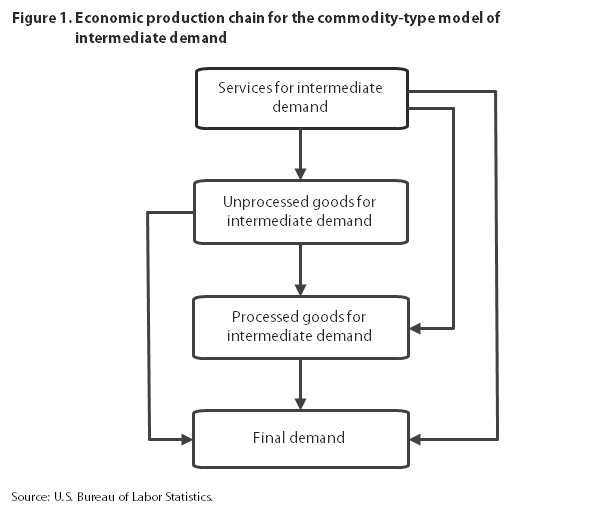
Intermediate-demand services are found first in the production chain because they are likely inputs to all other types of products; by contrast, in most cases, other product types are not substantial inputs to intermediate-demand services. Unprocessed goods for intermediate demand are second, since they can be inputs to processed goods for intermediate or final demand, but neither processed goods for intermediate demand nor final-demand products are a significant source of inputs to unprocessed goods for intermediate demand. Processed goods for intermediate demand are third, because they are inputs to final-demand products, but not vice versa. The economic production chain ends with final-demand products, which are, by definition, not inputs to any of the products included at earlier stages of the model.
A VAR model can be used to examine the nature of causal price-transmission relationships among the indexes for intermediate demand by commodity type and the indexes for final demand. VAR modeling involves estimating a system of equations in which each variable is expressed as a linear combination of lagged values of itself and all other variables in the system.8 A four-variable VAR was estimated from the PPIs for services for intermediate demand, unprocessed goods for intermediate demand, processed goods for intermediate demand, and final demand. The estimation used monthly data from October 2009 through December 2014. (FD–ID data series typically begin in October 2009.) All data were seasonally adjusted and converted to month-to-month percentage-growth form.
A time series is stationary if the mean, variance, and covariance of the series are not dependent on time. The estimation of a VAR with nonstationary data is problematic, because the tests used to estimate the significance of the VAR coefficients in such a procedure would not be valid. To test for stationarity, the Dickey–Fuller test was applied; in this one-tailed test, the null hypothesis is that the time series is not stationary. A large negative test statistic would reject the null hypothesis and imply that the time series is stationary.9 Dickey–Fuller tests performed on the indexes for final demand and intermediate demand by commodity type indicated that, when the data are converted to percentage-growth form, all of the time series are stationary. To determine the correct lag structure of the VAR, the Schwarz information criterion was implemented.10 The criterion suggested that a VAR whose equations have one lag is optimal; therefore, the VAR was estimated with the use of one lag of each variable.
The VAR model was first used to test for Granger causality among the indexes. A variable is said to Granger-cause a second variable when adding past values of the variable to an autoregressive model of the second variable improves the predictability of the latter. Wald statistics were used to test the null hypothesis of no Granger causality. Wald tests are based on measuring the extent to which the unrestricted estimates fail to satisfy the restrictions of the null hypothesis. A small p-value of the Wald statistic would reject the null hypothesis of no feedback to the dependent variable, and a large p-value of the Wald statistic would imply that the null hypothesis is not rejected. A p-value of less than 0.01 would reject the null hypothesis at the 99-percent confidence level, whereas a p- value of 0.05 or less would do so at the 95-percent confidence level. P-values greater than 0.05 would suggest acceptance of the null hypothesis of no Granger causality.11
In addition to testing for Granger causality from individual indexes to the dependent variable, the analysis included Granger-causality tests of joint lagged values of all variables that would precede or follow the dependent variable in the economic production chain outlined in figure 1. For example, the null hypothesis that prices for services, unprocessed goods, and processed goods for intermediate demand do not jointly Granger-cause final-demand prices was tested. The results of the Granger-causality tests are presented in table 1.
| Null hypothesis | Chi-square | p-value |
|---|---|---|
Dependent variable: Services for ID | ||
Unprocessed goods for ID = 0 | 0.205 | 0.651 |
Processed goods for ID = 0 | 1.491 | .222 |
Final demand = 0 | .258 | .611 |
Unprocessed goods for ID, processed goods for ID, and final demand = 0 | 3.913 | .271 |
Dependent variable: Unprocessed goods for ID | ||
Services for ID = 0 | .056 | .812 |
Processed goods for ID = 0 | .748 | .387 |
Final demand = 0 | 1.311 | .252 |
Processed goods for ID and final demand = 0 | 1.315 | .518 |
Dependent variable: Processed goods for ID | ||
Services for ID = 0 | .012 | .913 |
Unprocessed goods for ID = 0 | 5.273 | .022(1) |
Services for ID and unprocessed goods for ID = 0 | 5.296 | .071 |
Final demand = 0 | .325 | .569 |
Dependent variable: Final demand | ||
Services for ID = 0 | .077 | .782 |
Unprocessed goods for ID = 0 | 6.213 | .013(1) |
Processed goods for ID = 0 | 5.496 | .019(1) |
Services for ID, unprocessed goods for ID, and processed goods for ID = 0 | 20.477 | .000(2) |
| Notes: (1) Significant at the 95-percent confidence level. (2) Significant at the 99-percent confidence level. Note: ID = Intermediate demand. Source: Author's calculations based on data from the U.S. Bureau of Labor Statistics. | ||
The Granger-causality tests suggest that price changes for less processed intermediate-demand goods are passed forward to more processed intermediate-demand goods and to final demand, but that price changes for intermediate-demand services are not passed through to intermediate-demand goods or to final demand. The tests show that the index for unprocessed goods for intermediate demand Granger-causes both the index for processed goods for intermediate demand and the index for final demand. Moreover, prices for processed goods for intermediate demand Granger-cause final-demand prices, and prices for unprocessed goods for intermediate demand, processed goods for intermediate demand, and intermediate-demand services jointly Granger-cause final-demand prices. In no instance does the index for intermediate-demand services alone Granger-cause any other variables in the system. The tests also suggest that price changes for final demand do not lead to changes in intermediate-demand prices, as the final-demand index does not Granger-cause any intermediate-demand indexes included in the model.
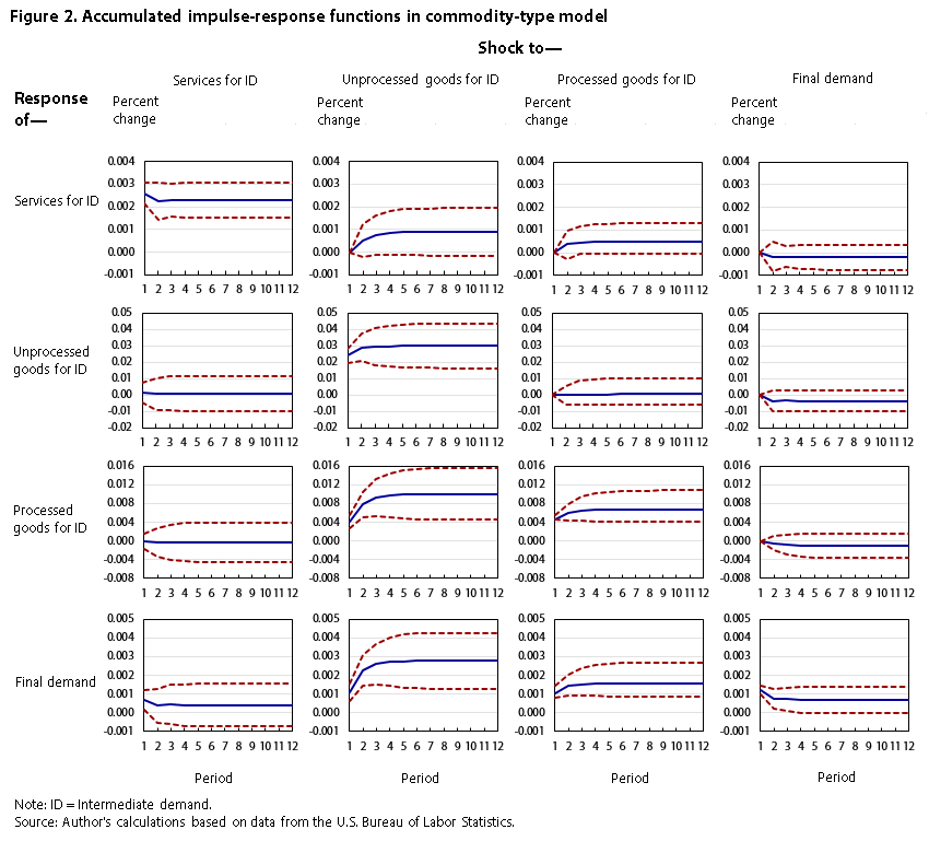
VAR coefficients are difficult to interpret because of the multivariate nature of the models. Accordingly, impulse-response functions and variance decompositions were developed to assist in interpreting the VARs.12 Impulse-response functions measure the effect of a one-standard-deviation perturbation of a variable in a system of equations on current and future values of all variables in the system. Variance decompositions show the percentage of forecast-error variance in one variable of the VAR that is explained by perturbations to all variables used in the VAR.13 Because shocks within a VAR are generally contemporaneously correlated, a random shock to one variable often occurs simultaneously with shocks to other variables. To overcome this problem, the residuals may be orthogonalized by a Cholesky decomposition in which the covariance matrix of the residuals is lower triangular. In this decomposition, a shock to one variable in the system contemporaneously affects only variables ordered after that variable in the VAR, and the VAR is given a causal interpretation.14 To calculate the impulse-response functions and variance decompositions of variables in the commodity-type model, the residuals were orthogonalized by a Cholesky decomposition using the following ordering of commodities: services for intermediate demand, unprocessed goods for intermediate demand, processed goods for intermediate demand, final demand. This ordering was chosen because economic theory predicts that price changes for inputs costs would be passed forward to more processed products.
Figure 2 presents the accumulated impulse-response functions of one-standard-deviation shocks to the indexes for services for intermediate demand, unprocessed goods for intermediate demand, processed goods for intermediate demand, and final demand. To represent the statistical significance of the impulse-response functions, standard-error bands (dashed red lines) were constructed with the use of the software program EViews 5.0.15 The impulse responses are significant at the 95-percent confidence level when both standard-error bands are simultaneously above or below zero on the y-axis.
The accumulated impulse-response functions indicate that, within the commodity-type model, price changes for less processed goods are passed forward to more processed commodities. An unanticipated change to the index for unprocessed goods for intermediate demand significantly affects prices for both processed goods for intermediate demand and final demand. Likewise, a shock to the index for processed goods for intermediate demand leads to significant changes in the index for final demand. The impulse-response functions also provide modest support for the notion that changes in prices for intermediate-demand services are passed onto final-demand prices, because an unanticipated change in the index for services for intermediate demand leads to a marginally significant change in the final-demand index. The impulse-response functions do not indicate that changes in final-demand prices are transmitted to commodities found earlier in the production chain, or that prices for partially processed intermediate-demand goods are transmitted backward to prices for unprocessed goods. A shock to the index for final demand does not lead to significant changes to any other variables in the model, and unanticipated changes in the index for processed goods for intermediate demand do not lead to significant changes in the index for unprocessed goods for intermediate demand.
Table 2 presents the variance decompositions of the commodity-type indexes after 12 months.16 The variance decompositions reinforce the earlier finding that changes in final-demand prices are affected by price changes for intermediate-demand commodities. Unanticipated changes in prices for services for intermediate demand, unprocessed goods for intermediate demand, and processed goods for intermediate demand account for, respectively, about 9, 43, and 21 percent of the forecast-error variance in the index for final demand. The variance decompositions also indicate that changes in processed-goods prices can result from changes in unprocessed-goods prices, because shocks to unprocessed-goods prices account for approximately 58 of the forecast-error variance in the index for processed goods for intermediate demand. Finally, the variance decompositions show that very little of the forecast-error variance in either the indexes for services for intermediate demand or the indexes for unprocessed goods for intermediate demand can be attributed to other variables in the model.
| Decomposition variable | Percentage of forecast errors due to— | |||
|---|---|---|---|---|
| Services for ID | Unprocessed goods for ID | Processed goods for ID | Final demand | |
Services for ID | 93.14 | 4.51 | 1.95 | 0.40 |
Unprocessed goods for ID | .48 | 97.48 | .02 | 2.02 |
Processed goods for ID | .09 | 57.96 | 41.34 | .60 |
Final demand | 8.77 | 43.40 | 20.55 | 27.29 |
Note: ID = Intermediate demand. Source: Author's calculations based on data from the U.S. Bureau of Labor Statistics. | ||||
The production-flow model of intermediate demand is a stage-based system of price indexes. It is constructed in a manner that maximizes forward flow of production between stages, while minimizing backward flow of production. It contains four main indexes: intermediate-demand stage 1, intermediate-demand stage 2, intermediate-demand stage 3, and intermediate-demand stage 4. Final demand can be added as the final stage in the model.
Indexes for the four intermediate-demand stages were developed by first assigning each industry in the economy to a stage. Industries assigned to the fourth stage produce output primarily consumed as final demand, industries in the third stage produce output primarily consumed by stage-4 industries, industries assigned to the second stage produce output primarily consumed by stage-3 industries, and industries assigned to the first stage produce output primarily consumed by stage-2 industries. Production-flow indexes track prices for the net inputs consumed by industries in each of the four stages of production. For example, the stage-4 intermediate-demand index tracks price changes for inputs consumed, but not produced, by industries included in the fourth stage of production. Hence, the stage-4 index measures price change in the inputs to production of industries that primarily produce final-demand commodities. The main sources of data used to develop these indexes were the Bureau of Economic Analysis “Use of commodities by industries, before redefinition” and “Make of commodities by industries, before redefinition” tables.17
In order to examine the nature of causal price-transmission relationships among the intermediate-demand-by-production-flow indexes and the final-demand indexes, a four-variable VAR was estimated with the use of monthly data from October 2009 through December 2014. The estimation included PPIs for stage-2 intermediate demand, stage-3 intermediate demand, stage-4 intermediate demand, and final demand. The stage-1 intermediate-demand index was omitted from the model because the transactions included at this stage are, by construction, backflow from earlier stages in the system, making stage 1 less useful for price-transmission analysis. All indexes were seasonally adjusted and converted to month-to-month percentage-growth form. Dickey-Fuller tests indicated that, when the data are converted to percentage growth form, all of the time series involved are stationary. To determine the correct lag structure of the VAR, the Schwarz information criterion was implemented. Again, the criterion suggested that a VAR whose equations have one lag is optimal; therefore, one lag of each variable was used to estimate the VAR.
Granger-causality tests were performed with the use of the VAR model. In addition to testing for Granger causality from individual indexes to the dependent variable, the analysis tested joint lagged values of all variables at stages of processing before and after the stage of the dependent variable. For example, the null hypothesis that prices for stage-2 and stage-3 intermediate demand do not jointly Granger-cause stage-4 intermediate demand was tested. Table 3 presents the results of the Granger-causality tests for the production-flow model.
| Null hypothesis | Chi-square | p-value |
|---|---|---|
Dependent variable: Stage-2 ID | ||
Stage-3 ID = 0 | 3.279 | 0.070 |
Stage-4 ID = 0 | .543 | .461 |
Final demand = 0 | .034 | .853 |
Stage-3 ID, stage-4 ID, and final demand = 0 | 3.667 | .300 |
Dependent variable: Stage-3 ID | ||
Stage-2 ID = 0 | 4.001 | .046(1) |
Stage-4 ID = 0 | .635 | .426 |
Final demand = 0 | 1.339 | .247 |
Stage-4 ID and final demand = 0 | 1.363 | .506 |
Dependent variable: Stage-4 ID | ||
Stage-2 ID = 0 | 4.523 | .033(1) |
Stage-3 ID = 0 | .986 | .321 |
Stage-2 ID and stage-3 ID = 0 | 5.851 | .054 |
Final demand = 0 | .803 | .370 |
Dependent variable: Final demand | ||
Stage-2 ID = 0 | 2.220 | .136 |
Stage-3 ID = 0 | 5.004 | .025(1) |
Stage-4 ID = 0 | .005 | .943 |
Stage-2 ID, stage-3 ID, and stage-4 ID = 0 | 13.623 | .004(2) |
| Notes: (1) Significant at the 95-percent confidence level. (2) Significant at the 99-percent confidence level. Note: ID = Intermediate demand. Source: Author's calculations based on data from the U.S. Bureau of Labor Statistics. | ||
The Granger-causality tests show that price changes at each stage of production are explained by changes in prices at earlier stages of production, and not explained by prices at later stages of production. In no equation is an explanatory variable (or a combination of explanatory variables) significant if its stage of production follows that of the dependent variable. By contrast, the stage-2 intermediate-demand index Granger-causes the indexes for both stage-3 intermediate demand and stage-4 intermediate demand. Moreover, the stage-3 intermediate-demand index Granger-causes the final-demand index, and the indexes for intermediate demand at stages 2, 3, and 4 jointly Granger-cause the index for final demand.
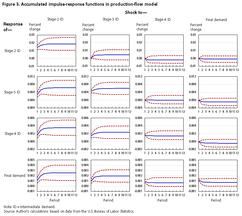
As in the previous model, impulse-response functions and variance decompositions were constructed from an orthogonalized set of residuals. This was done with the use of a Cholesky decomposition based on the following ordering: stage-2 intermediate demand, stage-3 intermediate demand, stage-4 intermediate demand, final demand. This ordering was chosen because economic theory predicts that input price changes would be passed on to higher-level producers in the production chain. In addition, the Granger-causality tests suggest that this ordering is correct. The accumulated impulse-response functions are presented in figure 3.
The accumulated impulse-response functions indicate that price changes within the production-flow model are passed forward through the stages of production. In every instance, an unanticipated price change at an earlier stage of the model results in significant price changes at later stages. For example, a shock to the index for stage-2 intermediate demand results in significant movements in the indexes for stage-3 intermediate demand, stage-4 intermediate demand, and final demand. Likewise, an unanticipated change in prices for stage-3 intermediate demand leads to significant changes in prices for stage-4 intermediate demand and for final demand. The impulse-response functions also imply that price movements are not passed backward through the stages of processing. In no instance does a price shock at a later stage of production lead to significant price movements at earlier stages.
Variance decompositions also suggest that price changes are passed forward, as opposed to backward, through the stages of the production-flow model. Table 4 shows that approximately 35, 25, and 15 percent of the forecast-error variance in the index for final demand are attributable to unanticipated changes in the indexes for stage-2 intermediate demand, stage-3 intermediate demand, and stage-4 intermediate demand, respectively. Unanticipated changes in the indexes for stage-2 intermediate demand and stage-3 intermediate demand account for 47 and 27 percent, respectively, of the forecast-error variance in the stage-4 intermediate-demand index, whereas shocks to final-demand prices account for only 1 percent of the forecast-error variance. Approximately 40 percent of the forecast-error variance in the stage-3 intermediate-demand index is explained by unexpected changes in the index for stage-2 intermediate demand, whereas innovations to prices for stage-4 intermediate demand and final demand explain very little of the forecast-error variance in the stage-3 intermediate-demand index. Finally, more than 90 percent of the forecast-error variance in the stage-2 intermediate-demand index can be attributed to unexpected changes in that index itself.
| Decomposition variable | Percentage of forecast errors due to— | |||
|---|---|---|---|---|
| Stage-2 ID | Stage-3 ID | Stage-4 ID | Final demand | |
Stage-2 ID | 91.72 | 6.22 | 1.88 | 0.18 |
Stage-3 ID | 39.51 | 58.68 | .07 | 1.73 |
Stage-4 ID | 46.70 | 26.69 | 25.56 | 1.05 |
Final demand | 35.19 | 24.64 | 14.62 | 25.55 |
Note: ID = Intermediate demand. Source: Author's calculations based on data from the U.S. Bureau of Labor Statistics. | ||||
This article presented an empirical investigation of the nature of causal price relationships within the new PPI FD–ID system. Using two separate VAR models, the analysis examined causal relationships between the index for final demand and indexes for two PPI treatments of intermediate demand: commodity type and production flow.
The first VAR model was used to examine price transmission among the intermediate-demand-by-commodity-type indexes and the index for final demand. Impulse-response functions developed from the VAR model’s coefficients indicated that price changes for less processed goods are passed forward to more processed commodities. The impulse-response functions also provided modest support for the notion that changes in prices for intermediate-demand services are passed onto other types of commodities. The impulse-response functions did not indicate that changes in final-demand prices are transmitted to commodities found earlier in the production chain, or that prices for partially processed intermediate-demand goods are transmitted backward to prices for unprocessed goods. Variance decompositions told a similar story. Substantial portions of the forecast-error variance in the index for final demand were explained by unanticipated changes in the indexes for all types of intermediate-demand commodities: unprocessed goods, processed goods, and services. Likewise, a large portion of the forecast-error variance in the index for processed goods for intermediate demand was accounted for by innovations in the index for unprocessed goods for intermediate demand.
The second VAR model was used to analyze the causal price relationships between the intermediate-demand-by-production-flow indexes and the index for final demand. Impulse-response functions from the VAR indicated that price changes are transmitted forward, but not backward, through the production-flow stages. In every instance, an unanticipated price shock resulted in a statistically significant change in prices at stages ahead of where the shock occurred. By contrast, in no case did a price shock lead to a significant change in prices at an earlier stage of the production-flow model. Variance decompositions also showed that price changes are passed forward, but not backward, through the stages of the model. A substantial portion of the forecast-error variance at every stage was accounted for by unanticipated changes in prices at earlier stages, but not later stages.
Although the VAR models constructed from both the commodity-type and production-flow indexes indicated forward price transmission, the causal relationships were clearer and stronger in the production-flow model. Within that model, shocks to prices at earlier stages always produced significant changes to prices at later stages, and price changes were never significantly transmitted backward through the stages. Within the commodity-type model, price changes were transmitted forward to more processed commodities in most, but not all, cases. The clearer price transmission seen in the production-flow model is somewhat expected, because that model was constructed with the explicit goal of maximizing forward flow of production between stages while minimizing backward flow.
Overall, the results of this article confirm that the commodity-type and production-flow models of intermediate demand are measuring price transmission as they were intended to do when they were first conceptualized and constructed by BLS.
Jonathan C. Weinhagen, "Price transmission within the Producer Price Index Final Demand–Intermediate Demand aggregation system," Monthly Labor Review, U.S. Bureau of Labor Statistics, August 2016, https://doi.org/10.21916/mlr.2016.33
1 The PPI definition of commodities includes goods, services, and construction products.
2 For a detailed description of the PPI FD–ID system, see Jonathan C. Weinhagen, “A new, experimental system of indexes from the PPI program,” Monthly Labor Review, February 2011, pp. 3–24, https://www.bls.gov/opub/mlr/2011/02/art1full.pdf.
3 S. Brock Blomberg and Ethan S. Harris, “The commodity–consumer price connection: fact or fable?” Federal Reserve Bank of New York Economic Policy Review, October 1995, pp. 21–38, https://www.newyorkfed.org/medialibrary/media/research/epr/95v01n3/9510blom.pdf.
4 Fred Furlong and Robert Ingenito, “Commodity prices and inflation,” Federal Reserve Bank of San Francisco Economic Review, no. 2, 1996, pp. 27–47, http://www.frbsf.org/economic-research/files/furlong.pdf.
5 Todd E. Clark, “Do producer prices lead consumer prices?” Federal Reserve Bank of Kansas City Economic Review, third quarter, 1995, pp. 26–39, https://www.kansascityfed.org/documents/1005/1995-Do%20Producer%20Prices%20Lead%20Consumer%20Prices%3F.pdf.
6 Tae-Hwy Lee and Stuart Scott, “Investigating inflation transmission by stages of processing,” in Robert F. Engle and Halbert White, eds., Cointegration, causality, and forecasting: a festschrift in honor of Clive W. J. Granger (Oxford, UK: Oxford University Press, August 1999), pp. 283–300.
7 Jonathan C. Weinhagen, “An empirical analysis of price transmission by stage of processing,” Monthly Labor Review, November 2002, pp. 3–11, https://www.bls.gov/opub/mlr/2002/11/art1full.pdf; and Jonathan C. Weinhagen, “Price transmission within the PPI for intermediate goods,” Monthly Labor Review, May 2005, pp. 41–49, https://www.bls.gov/opub/mlr/2005/05/art4full.pdf.
8 William Greene, Econometric analysis (Upper Saddle River, NJ: Prentice-Hall Inc., 1997), see especially pp. 815–816.
9 David A. Dickey and Wayne A. Fuller, “Distribution of the estimators for autoregressive time series with a unit root,” Journal of the American Statistical Association, vol. 74, no. 366, 1979, pp. 427–431.
10 Philip Hans Franses, Time series models for business and economic forecasting (Cambridge, UK: Cambridge
University Press, 1998).
11 Greene, Econometric analysis, p. 161.
12 Christopher A. Sims, “Macroeconomics and reality,” Econometrica, January 1980, pp.1–48.
13 John Dinardo and Jack Johnston, Econometric methods (New York: McGraw Hill, 1996), pp. 289–301.
14 Ibid.
15 EViews 5 user’s guide (Quantitative Micro Software, LLC, April 15, 2004), p. 714.
16 Walter Enders, Applied econometric time series (Hoboken, NJ: John Wiley & Sons, Inc., 2004), pp. 278–280.
17 BEA input–output accounts data can be found at https://www.bea.gov/industry/io_annual.htm.