An official website of the United States government
An official website of the United States government
The .gov means it's official.
Federal government websites often end in .gov or .mil. Before sharing sensitive information,
make sure you're on a federal government site.
The site is secure.
The
https:// ensures that you are connecting to the official website and that any
information you provide is encrypted and transmitted securely.
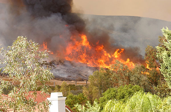
The severity and destruction of wildfires in California have increased in magnitude every decade since the late 1900s. Some researchers have studied the impacts of wildfires on people’s health and earnings and on the environment, but few have studied their impacts on the labor market. In this article, I estimate the impacts of destructive wildfires on short-term employment changes by using a generalized difference-in-difference modeling approach with an event-study specification (impacts of an event over time). Although the impacts are small at the overall (cross-industry) level, the analysis of this article shows that specific industries generally had much larger impacts during the analysis period of 2003 through 2021. For example, construction, the most visibly affected industry, had a statistically significant employment growth rates of from 5 percent to 10 percent for at least 18 months postfire. Professional and business services also had significant employment growth rates of up to 5 percent for at least 18 months postfire.
California has a long history of wildfires. In each decade between 1960 and 1990, wildfires destroyed fewer than 1,000 structures.[1] In the 1990s, that number rose to over 6,000 and then increased further to over 10,000 in the first decade of the new millennium.[2] In the 2010s, that figure jumped to over 50,000, with the Tubbs Fire in 2017 destroying over 5,600 structures and the Camp Fire in 2018 destroying nearly 19,000 structures.[3] Rising temperatures, drier weather conditions, and increased construction of housing and infrastructure in the expanding wildland-urban interface are contributing to the increased wildfire prevalence and severity.[4] California wildfires have received much attention, in part, not only because of the severity of the events but also because of the adverse air quality from wildfire smoke that affects populations far from the fires themselves, causing potential health issues, financial impacts, and water-quality challenges.[5]
Much of the literature surrounding labor market impacts of natural disasters has focused on events such as tsunamis, earthquakes, hurricanes, and tornadoes.[6] Many studies have found that wages increased and employment fell postevent, depending on the severity of a natural disaster. Employment and wage changes may be due to combinations of rebuilding activity, outmigration, and sector-level effects. Although some studies have focused on the effects of large wildfires on labor market outcomes,[7] not one has studied the employment impacts of different-sized wildfires by industry sectors in California.
In this article, the analysis uses the panel data structure of multiple wildfire events across time in multiple counties in California and uses a generalized difference-in-difference (GDD) modeling approach with an event-study specification (impacts of an event over time) for measuring the effects of destructive wildfires on labor markets over time.[8] Differences across each of the 10 major industry sectors are also discussed.
California fire incident data from the California Department of Forestry and Fire Protection (CalFire) between January 2003 and March 2021 are aggregated at the county level and merged with monthly employment data from the U.S. Bureau of Labor Statistics (BLS) Quarterly Census of Establishment and Wages (QCEW). The data are merged at the county-by-month level.
This article uses a dataset of about 600 individual records of fire events between January 2003 and March 2021 that exceeded 1,000 acres. The dataset was extracted from CalFire and other administrative unit agencies for non-CalFire incidents. The assembled dataset includes the name of fires, counties, start and end dates, acres of event, and number of destroyed structures. This list is then aggregated to the county-by-month level.
California statewide and county-level monthly data between January 2003 and March 2021 are used.[9] The dataset includes only private establishments (it excludes local, state, or federal government). Because of the heterogeneous seasonality across counties and industries, these data are first seasonally adjusted with the use of X-12-ARIMA that stabilizes the variance at the statewide, statewide by industry, county, and county by industry levels.[10] Other common standard practices in the literature include adding seasonal controls directly into the model for some longitudinal data. However, for this dataset, because of the heterogeneous seasonality across counties and industries, broad seasonal controls do not sufficiently capture these microseasonality differences.[11] Counties with a population under 50,000 are excluded from the analysis because of data limitations.[12]
To measure the extent of damage from a fire event at the county level, I weigh the number of destroyed structures by the county population, that is, the number of destroyed structures per 1,000 county population,[13] or the local destruction index (LDI). Destructive fires that affect large acreage but few structures or fire events that destroy many structures but in a populous county may not have a large LDI. Furthermore, the analysis in this article defines the size of a wildfire by a combination of LDI and minimum number of structures destroyed:
· “Large” are those fires with an LDI greater than or equal to 1.0 and that destroy 300 or more structures.
· “Medium” are those fires with an LDI greater than or equal to 0.1 and that destroy 100 or more structures and are not large.
· “Small” are those fires with an LDI greater than or equal to 0.01 and that destroy 10 or more structures or equal to 10 and are not large or medium.
Fires that have less than 10 destroyed structures or have an LDI less than 0.01 are measurably indistinguishable from no fires and together form the baseline group.
To form a more comparable set of counties and months, the analysis further restricts the data to only counties that are most prone to wildfires. Counties that have above-average rates of significant fires (fires that burned over 1,000 acres) over the 18-year analysis period are used. Furthermore, the data are further restricted to only the core wildfire season months, June through October. Analysis for the full dataset was also run as part of robustness checks (see the section that follows), and results were mostly unchanged.
The number of fires greater than 1,000 acres has trended upward in the past two decades. (See chart 1.) Wildfire season may start as early as May, peaks in July and August, and can last through the fourth quarter. (See chart 2.)
| Year | Number of fires |
|---|---|
| 2003 | 11 |
| 2004 | 12 |
| 2005 | 9 |
| 2006 | 38 |
| 2007 | 36 |
| 2008 | 29 |
| 2009 | 29 |
| 2010 | 10 |
| 2011 | 25 |
| 2012 | 34 |
| 2013 | 26 |
| 2014 | 32 |
| 2015 | 32 |
| 2016 | 38 |
| 2017 | 77 |
| 2018 | 51 |
| 2019 | 31 |
| 2020 | 53 |
| Source: California Department of Forestry and Fire Protection, https://www.fire.ca.gov/. | |
| Month | Acres burned | Number of fires greater than 1,000 acres |
|---|---|---|
| Jan | 1,952 | 1 |
| Feb | 21,154 | 4 |
| Mar | 6,136 | 2 |
| Apr | 12,895 | 6 |
| May | 193,789 | 37 |
| Jun | 851,064 | 86 |
| Jul | 3,394,905 | 139 |
| Aug | 4,508,619 | 136 |
| Sep | 1,645,412 | 87 |
| Oct | 1,482,308 | 52 |
| Nov | 322,604 | 13 |
| Dec | 336,380 | 10 |
| Source: California Department of Forestry and Fire Protection, https://www.fire.ca.gov/. | ||
The map on the left in chart 3 shows the annual average number of structures destroyed by county between 2015 and 2020. Of 58 California counties, 26 counties had an average of 10 or more destroyed structures per year between 2015 and 2020. Fires occurred throughout California, but Northern California counties appear to have suffered from larger and more frequent wildfires. At the more extreme end, Butte County had an average of more than 3,000 destroyed structures per year, whereas Napa County had an average of 2,000 destroyed structures.
Source: California Department of Forestry and Fire Protection https://www.fire.ca.gov/ and U.S. Census Bureau.
| County | Destruction index | Destroyed structures |
|---|---|---|
| Alameda County | 0.0 | 0 |
| Alpine County | 0.0 | 0 |
| Amador County | 4.0 | 154 |
| Butte County | 13.8 | 3,174 |
| Calaveras County | 0.0 | 0 |
| Colusa County | 2.1 | 47 |
| Contra Costa County | 0.0 | 0 |
| Del Norte County | 0.0 | 0 |
| El Dorado County | 0.0 | 0 |
| Fresno County | 0.2 | 158 |
| Glenn County | 0.0 | 0 |
| Humboldt County | 0.0 | 1 |
| Imperial County | 0.0 | 0 |
| Inyo County | 0.4 | 8 |
| Kern County | 0.1 | 57 |
| Kings County | 0.0 | 0 |
| Lake County | 7.0 | 450 |
| Lassen County | 0.1 | 5 |
| Los Angeles County | 0.0 | 363 |
| Madera County | 0.0 | 3 |
| Marin County | 0.0 | 0 |
| Mariposa County | 1.5 | 27 |
| Mendocino County | 3.0 | 263 |
| Merced County | 0.0 | 0 |
| Modoc County | 0.0 | 0 |
| Mono County | 0.0 | 0 |
| Monterey County | 0.1 | 35 |
| Napa County | 14.2 | 1,997 |
| Nevada County | 0.0 | 1 |
| Orange County | 0.0 | 30 |
| Placer County | 0.0 | 0 |
| Plumas County | 26.2 | 492 |
| Riverside County | 0.0 | 20 |
| Sacramento County | 0.0 | 0 |
| San Benito County | 0.0 | 0 |
| San Bernardino County | 0.0 | 69 |
| San Diego County | 0.0 | 52 |
| San Francisco County | 0.0 | 0 |
| San Joaquin County | 0.0 | 0 |
| San Luis Obispo County | 0.1 | 19 |
| San Mateo County | 0.0 | 0 |
| Santa Barbara County | 0.5 | 232 |
| Santa Clara County | 0.0 | 46 |
| Santa Cruz County | 1.0 | 272 |
| Shasta County | 1.8 | 327 |
| Sierra County | 0.6 | 2 |
| Siskiyou County | 0.4 | 16 |
| Solano County | 0.0 | 1 |
| Sonoma County | 0.1 | 74 |
| Stanislaus County | 0.1 | 34 |
| Sutter County | 0.0 | 0 |
| Tehama County | 0.1 | 4 |
| Trinity County | 0.7 | 9 |
| Tulare County | 0.0 | 1 |
| Tuolumne County | 0.4 | 23 |
| Ventura County | 0.0 | 3 |
| Yolo County | 0.0 | 2 |
| Yuba County | 0.7 | 55 |
| Source: California Department of Forestry and Fire Protection https://www.fire.ca.gov/ and U.S. Census Bureau. | ||
The map on the right in chart 3 shows the annual average LDI. Ten counties had an LDI higher than 1, that is, more than 1 destroyed structure annually per 1,000-county population. At the extreme end, both Butte and Napa Counties had an LDI of 14. Plumas County, a smaller county (with population less than 20,000) with many destroyed structures (nearly 500), had the highest LDI of 26.[14] All three counties are located in Northern California.
For estimating how an outcome would differ since an event occurred as compared with if no event had occurred, a generalized difference-in-difference (GDD) modeling approach is used with an event-study specification. The GDD approach estimates the impact of exogenous shocks, such as wildfires, on employment over time, by comparing employment in counties and periods with wildfires with employment in counties without wildfires. However, unlike a standard GDD approach in which a single difference (such as first differences or 12-month difference) is used and only measures the impact of an event in the month of the event,[15] separate +h-difference models are estimated in an event-study setup in which h goes from 0 through 18 months. This method allows estimation of the temporal impacts of wildfire events. That is, the impacts of wildfires on employment are estimated for each month after the event for 18 months,[16] as compared with the period before the fire (t – 1). The degenerate case of h=0 is a standard first difference in a GDD model and measures the impact of an event in the month of the event.
As with standard panel data analysis, the analysis first pools (or stacks) the cross-sectional data (counties) across time (months or quarters) and denotes the labor market outcomes, Y (relative employment percent change), in county, c, at time, t, by Yct. Since growth rates of the outcomes between two periods—the month before an event (t – 1) and h-months after an event (t + h)—are examined, the natural log of Yct is used and rewritten as h+1-differences:  ln Yc,t+h − ln Yc,t−1, where h goes from 0 to 18. Similarly, this h+1-month difference for California statewide is computed and then removed from each county as a general state-level business cycle detrending.[17] This detrended percent change is defined as
  .
.
The empirical model is expressed as

where L, M, and S are indicators for large, medium, and small fire events. The main coefficients of interest are  ,
,  , and
, and  and represent the beyond expected percent change (as compared with periods of no fires) in a labor market outcome relative to the period before an event, h months after a fire event. For example, changes in employment 1 year after a fire event for counties that had large fires are compared with employment changes of all 1-year periods in all counties where no fire event occurred. Also, γk captures the coefficients on k-period-lagged first differences, a way to capture and control for the effects of economic momentum. The analysis in this article estimates this model for all integer values of h from 0 through 18, that is, for each month up to 18 months since a potential fire event. The variation in the error term comes from randomness in timing and counties. In the model just described, the counties and periods after a fire event are the “treatment” group and the counties and/or periods without a fire event are the “control” group.
After the transformation of these data, the model is estimated by using ordinary least squares procedures for each outcome and h. For conciseness and more general results, these estimates are averaged into quarterly categories. For example, “Q1” (quarter 1) indicates the average of months 1 through 3 following the month of a fire event, Q2 (quarter 2) indicates the average of months 4 through 6 following the month of a fire event, and so forth.
For each of the summarized estimates of the time categories, standard errors are computed via bootstrap resampling. For each recomputation, the fire-size indicators are sampled with replacement (randomly assigning) across counties and time. Bootstrap standard errors and 95-percent confidence intervals are formed from 10,000 replications. The idea is to form bootstrapped distributions of potential estimates such that the null hypothesis is that wildfires have no impact on the outcomes. The resulting bootstrapped distribution of estimates represents the potential values an estimate may take when no underlying impact exists from fires (randomly assigned across counties and time). Estimates from the model that fall in the lower or upper 2.5 percentile of the distribution indicate statistical significance at the 5-percent alpha level.
Small and medium wildfires have little measurable impact on the overall local employment changes. In the month of a large wildfire, overall employment drops slightly but recovers quickly afterward in the same quarter. These findings are similar to previous studies on the economic impacts of natural disasters, which also found a slight negative employment impact in the short term following hurricanes and tornados.[18] However, these relatively minor impacts on the overall labor market hide much larger dynamics at the industry sector levels, an issue rarely studied in the literature.
As seen with the overall results, small and medium wildfires have relatively small impacts on labor markets across most industries. Henceforth, this article will focus mainly on the impacts of large wildfires on industries and will only mention medium and small wildfires when they are important to the discussion. See results in table 1 for more details.
| Industry | Month of event | Quarters after large fire event | |||||
|---|---|---|---|---|---|---|---|
| Q1 | Q2 | Q3 | Q4 | Q5 | Q6 | ||
| All industries | –0.4 | 0.1 | 0.5 | 0.6 | 0.3 | 0.3 | 0.1 |
| Natural resources and mining | –0.8 | 0.3 | 0.2 | 1.2 | 2.3 | 2.8 | 1.5 |
| Construction: large fires | 1.3 | 3.7 | 5.0 | 6.7 | 8.5 | 9.5 | 9.0 |
| Construction: medium fires | –0.1 | 0.3 | 0.3 | 2.0 | 4.1 | 4.8 | 5.6 |
| Construction: small fires | 0.1 | 0.4 | 0.9 | 1.6 | 2.2 | 2.5 | 2.2 |
| Manufacturing | –0.4 | 0.0 | 0.7 | –0.8 | –1.3 | –0.1 | –0.6 |
| Trade, transportation, and utilities | 0.2 | 0.3 | 0.4 | 0.8 | 0.5 | 0.5 | 0.3 |
| Information | –1.7 | –3.0 | –3.4 | –5.4 | –5.8 | –6.6 | –6.1 |
| Financial activities | 0.0 | –0.3 | –0.7 | 0 | 0.8 | 1.1 | 1.2 |
| Professional and business services | 0.4 | 0.7 | 2.7 | 3.7 | 3.9 | 5.2 | 4.1 |
| Education and health services | –0.3 | –0.4 | –0.6 | –1.3 | –1.7 | –2.0 | –1.9 |
| Leisure and hospitality | 0.1 | 0.0 | 1.2 | 0.5 | –0.9 | –2.0 | –1.0 |
| Other services | 0.0 | –0.6 | 0.1 | 2.6 | 2.1 | 0.9 | 3.1 |
| Note: Bolded values indicate periods for which any deviations from zero were significant (α = 0.05) by using bootstrap resampling. Q = quarter. Source: Authors calculations using data from the California Department of Forestry and Fire Protection and BLS Quarterly Census of Employment and Wages. | |||||||
During the 2003 through 2021 period, construction had the largest and most persistent employment growth rates following a large destructive wildfire. (See table 1.) As one would expect, if a large number of structures are destroyed in a community, an influx of construction workers is required to help rebuild the community. Following large wildfires, the number of construction workers steadily grew in the first 18 months to nearly 10 percent above what is expected normally without a fire. Medium and small fires also had a measurable impact on employment, with growths up to 5 percent and 3 percent, respectively, within the first 18 months.
Reconstruction and cleanup efforts, insurance payouts, as well as government funding may have contributed to a positive and sustained construction employment response.[19] These results are consistent with other natural disaster studies, which find that construction employment increases in the 2 years following a destructive earthquake.[20] (See chart 4.)
| Months since fire event | Small | Medium | Large |
|---|---|---|---|
| 0 | 0.1 | −0.1 | 1.3 |
| 1 | 0.3 | 0.0 | 1.7 |
| 2 | 0.4 | 0.4 | 4.8 |
| 3 | 0.5 | 0.6 | 4.7 |
| 4 | 0.7 | −0.1 | 5.2 |
| 5 | 0.9 | 0.5 | 4.9 |
| 6 | 1.2 | 0.4 | 5.0 |
| 7 | 1.5 | 0.8 | 6.0 |
| 8 | 1.5 | 2.1 | 6.5 |
| 9 | 1.7 | 3.0 | 7.4 |
| 10 | 2.0 | 3.4 | 7.7 |
| 11 | 2.2 | 4.0 | 9.1 |
| 12 | 2.2 | 5.0 | 8.8 |
| 13 | 2.4 | 4.8 | 10.6 |
| 14 | 2.4 | 4.5 | 9.8 |
| 15 | 2.5 | 5.3 | 8.1 |
| 16 | 2.1 | 5.6 | 7.6 |
| 17 | 2.3 | 5.5 | 9.0 |
| 18 | 2.2 | 5.8 | 10.4 |
| Source: California Department of Forestry and Fire Protection, https://www.fire.ca.gov/. | |||
Professional and business services employment also had a positive impact from large wildfires, with employment growths of up to 5 percent in the 18 months following a large fire event. Architectural and engineering services, which is part of the professional and business services industry, is another industry in which employment may have been affected in rebuilding homes and communities. As for other individual industries within the county of a fire, the impact of wildfires on employment was relatively minor, even with large wildfires.[21]
The analysis just discussed restricted data in several ways that included limiting data to only counties that had an above-average rate of significant fires and limiting data to only summer months to construct a most comparable group. The analysis was rerun with the full datasets (without these restrictions) as robustness checks. The results with the full dataset were similar to those of the restricted dataset. (See table 2.)
| Industry | Month of event | Quarters after large fire event | |||||
|---|---|---|---|---|---|---|---|
| Q1 | Q2 | Q3 | Q4 | Q5 | Q6 | ||
| All industries | –0.5 | –0.3 | 0.1 | –0.2 | –0.4 | –0.5 | –0.5 |
| Natural resources and mining | –0.8 | 0.3 | 0.8 | 0.6 | 1.9 | 2.8 | 2.9 |
| Construction: large fires | 0.4 | 2.4 | 4.6 | 5.4 | 6.5 | 6.8 | 6.4 |
| Construction: medium fires | –0.1 | 0.3 | 0.2 | 1.5 | 3.2 | 4.4 | 4.7 |
| Construction: small fires | 0.0 | 0.4 | 1.0 | 1.2 | 1.5 | 2.0 | 1.8 |
| Manufacturing | –0.3 | –0.2 | 0.6 | –0.7 | –1.4 | –0.6 | –0.7 |
| Trade, transportation, and utilities | –0.2 | 0.0 | 0.3 | 0.4 | 0.1 | 0.2 | 0.1 |
| Information | –1.7 | –3.8 | –4.8 | –6.4 | –6.1 | –6.0 | –4.8 |
| Financial activities | 0.1 | 0.1 | –0.6 | –0.3 | 0.2 | 0.4 | 0.8 |
| Professional and business services | –0.1 | 0.7 | 1.7 | 2.8 | 3.0 | 3.3 | 2.3 |
| Education and health services | –0.3 | –0.7 | –1.2 | –2.2 | –2.6 | –2.8 | –2.8 |
| Leisure and hospitality | –1.0 | –1.4 | –1.5 | –0.7 | –1.3 | –2.0 | –0.3 |
| Other services | -0.7 | –0.4 | –0.3 | 0.6 | 1.2 | 0.3 | 2.2 |
| Note: Bolded values indicate periods for which any deviations from zero were significant (α = 0.05) by using bootstrap resampling. Q = quarter. Source: Authors calculations using data from the California Department of Forestry and Fire Protection and BLS Quarterly Census of Employment and Wages. | |||||||
Wildfires have immediate impacts on people and local infrastructure but also have broader and longer-term impacts, including health, water, and local economies. Although the impacts of even large destructive wildfires seem minor on the aggregate local labor markets, their complex dynamics are much more pronounced at the sector level.
Large wildfires had a slight negative immediate impact on overall employment, which quickly recovered in the following months. These overall findings are generally consistent with some previous studies on the employment effects of natural disasters, such as earthquakes, tornados, hurricanes, and wildfires, which also found negative short-term employment growth.[22] Large wildfires, however, had a much higher impact on employment in particular industries. In the 2003 to 2021 period, construction employment saw growth of up to 10 percent in the first 18 months following a large wildfire. Professional and business services also saw employment growth of up to 5 percent in the same period. Understanding and predicting labor market changes after a natural disaster such as a destructive wildfire helps local businesses and governments plan for the changing needs of a local economy.
I thank Òscar Jordà, an economist at the Federal Reserve Bank of San Francisco and Economics Professor at University of California, Davis, for his invaluable guidance; and Michael Dalton, BLS research economist, and Mary Dorinda Allard, BLS assistant commissioner, both with the Office of Employment and Unemployment Statistics, for their review and comments.
Tian Luo, "Labor market impacts of destructive California wildfires," Monthly Labor Review, U.S. Bureau of Labor Statistics, July 2023, https://doi.org/10.21916/mlr.2023.16
1 Scott L Stephens, Mark A. Adams, John Handmer, Faith R. Kearns, Bob Leicester, Justin Leonard, and Max A. Moritz, “Urban–wildland fires: how California and other regions of the US can learn from Australia,” Environmental Research Letters, vol. 4, no. 1, February 2009, p. 2, https://doi.org/10.1088/1748-9326/4/1/014010.
2 Stephens et al., “Urban–wildland fires;” and California Department of Forestry and Fire Protection, “Current emergency incidents,” https://www.fire.ca.gov/incidents.
3 California Department of Forestry and Fire Protection, “Current emergency incidents,” https://www.fire.ca.gov/incidents.
4 Volker C. Radeloff, Roger B. Hammer, Susan I. Stewart, Jeremy S. Fried, Sheralyn S. Holcomb, and Jason F. McKeefry, “The wildland–urban interface in the United States,” Ecological Applications, vol. 15, no. 3, June 2005, pp. 799−805, https://doi.org/10.1890/04-1413; Volker C. Radeloff, David P. Helmers, H. Anu Kramer, Miranda H. Mockrin, Patricia M. Alexandre, Avi Bar-Massada, Van Butsic, Todd J. Hawbaker, Sebastián Martinuzzi, Alexandra D. Syphard, and Susan I. Stewart, “Rapid growth of the US wildland-urban interface raises wildfire risk,” Proceedings of the National Academy of Sciences, vol. 115, no. 13, March 2018, pp. 3,314−3,319, https://doi.org/10.1073/pnas.1718850115; Anthony L. Westerling, Hugo G. Hidalgo, Daniel R. Cayan, and Thomas W. Swetnam, “Warming and earlier spring increase western US forest wildfire activity,” Science, vol. 313, no. 5789, August 2006, pp. 940−943, https://doi.org/10.1126/science.1128834; Mike Flannigan, Alan S. Cantin, William J. de Groot, Mike Wotton, Alison Newbery, and Lynn M. Gowman, “Global wildland fire season severity in the 21st century,” Forest Ecology and Management, vol. 294, April 2013, pp. 54−61, https://doi.org/10.1016/j.foreco.2012.10.022; Anthony L. Westerling and Benjamin P. Bryant, “Climate change and wildfire in California,” Climatic Change, vol. 87, suppl. 1, 2008, pp. 231−249, https://doi.org/10.1007/s10584-007-9363-z; Jeremy S. Fried, Margaret S. Torn, and Evan Mills, “The impact of climate change on wildfire severity: a regional forecast for northern California,” Climatic Change, vol. 64, suppl. 1, May 2004, pp. 169−191, https://doi.org/10.1023/B:CLIM.0000024667.89579.ed; Max A. Moritz and Scott L. Stephens, “Fire and sustainability: considerations for California’s altered future climate,” Climatic Change, vol. 87, suppl. 1, 2008, pp. 265−271, https://doi.org/10.1007/s10584-007-9361-1; Scott L. Stephens, Jim K. Agee, Peter Z. Fulé, Malcolm P. North, William H. Romme, Thomas W. Swetnam, and Monica G. Turner, “Managing forests and fire in changing climates,” Science, vol. 342, no. 6154, October 2013, pp. 41−42, https://doi.org/10.1126/science.1240294; Donald McKenzie, Ze'ev Gedalof, David L. Peterson, and Philip Mote, “Climatic change, wildfire, and conservation,” Conservation Biology, vol. 18, no. 4, July 2004, pp. 890−902, https://doi.org/10.1111/j.1523-1739.2004.00492.x; Amy E. Hessl, “Pathways for climate change effects on fire: models, data, and uncertainties,” Progress in Physical Geography, vol. 35, no. 3, June 2011, pp. 393−407, https://doi.org/10.1177/0309133311407654; Mike D. Flannigan, Brian J. Stocks, and B. Mike Wotton, “Climate change and forest fires,” Science of the Total Environment, vol. 262, no. 3, November 2000, pp. 221−229, https://doi.org/10.1016/s0048-9697(00)00524-6; and Philip Gibbons, Linda van Bommel, A. Malcolm Gill, Geoffrey J. Cary, Don A. Driscoll, Ross A. Bradstock, Emma Knight, Max A. Moritz, Scott L. Stephens, and David B. Lindenmayer, “Land management practices associated with house loss in wildfires,” ed. Rohan H. Clarke, PLOS ONE [formerly PLoS ONE], vol. 7, no. 1, January 2012, https://doi.org/10.1371/journal.pone.0029212.
5 For health issues, see Neal Fann, Breanna Alman, Richard A Broome, Geoffrey G. Morgan, Fay H. Johnston, George Pouliot, and Ana G. Rappold, “The health impacts and economic value of wildland fire episodes in the US: 2008–2012,” Science of the Total Environment, vols. 610−611, January 2018, pp. 802−809, https://doi.org/10.1016/j.scitotenv.2017.08.024; Benjamin A. Jones, 2018, “Willingness to pay estimates for wildfire smoke health impacts in the US using the life satisfaction approach,” Journal of Environmental Economics and Policy, vol. 7, no. 4, April 2018, pp. 403−419, https://doi.org/10.1080/21606544.2018.1463872; Colleen E. Reid, Michael Brauer, Fay H. Johnston, Michael Jerrett, John R. Balmes, and Catherine T. Elliott, “Critical review of health impacts of wildfire smoke exposure,” Environmental Health Perspectives, vol. 124, no. 9, September 2016, pp. 1,334−1,343, https://doi.org/10.1289/ehp.1409277; Sarah B. Henderson and Fay H. Johnston, “Measures of forest fire smoke exposure and their associations with respiratory health outcomes,” Current Opinion in Allergy and Clinical Immunology, vol. 12, no. 3, June 2012, pp. 221−227, https://doi.org/10.1097/ACI.0b013e328353351f; and Martine Dennekamp and Michael J. Abramson, “The effects of bushfire smoke on respiratory health,” Respirology, vol. 16, no. 2, February 2011, pp. 198−209, https://doi.org/10.1111/j.1440-1843.2010.01868.x. For financial impacts, see Mark Borgschulte, David Molitor, and Eric Zou, “Air pollution and the labor market: evidence from wildfire smoke,” Working Paper 2528129952 (Cambridge, MA: National Bureau of Economic Research, April 2022), pp. 1,003−1,030; and Benjamin A. Jones and Shana McDermott, “The local labor market impacts of US megafires,” Sustainability, vol. 13, no. 16, August 2021, p. 9,078, https://doi.org/10.3390/su13169078. For water quality challenges, see Amanda K. Hohner, Charles C. Rhoades, Paul Wilkerson, and Fernando L. Rosario-Ortiz, “Wildfires alter forest watersheds and threaten drinking water quality,” Accounts of Chemical Research, vol. 52, no. 5, May 2019, pp. 1,234−1,244, https://doi.org/10.1021/acs.accounts.8b00670; Hohner et al., “Wildfires alter forest watersheds and threaten drinking water quality”; and Hugh G. Smith, Gary J. Sheridan, Patrick N.J. Lane, Petter Nyman, and Shane Haydon, “Wildfire effects on water quality in forest catchments: a review with implications for water supply,” Journal of Hydrology, vol. 396, nos. 1−2, January 2011, pp. 170−192, https://doi.org/10.1016/j.jhydrol.2010.10.043.
6 Ariel R. Belasen and Solomon W. Polachek, “How hurricanes affect wages and employment in local labor markets,” American Economic Review, vol. 98, no. 2, May 2008, pp. 49−53, https://doi.org/10.1257/aer.98.2.49; Ariel R. Belasen and Solomon W. Polachek, “How disasters affect local labor markets: the effects of hurricanes in Florida,” Journal of Human Resources, vol. 44, no. 1, January 2009, pp. 251−276, https://doi.org/10.3368/jhr.44.1.251; Eduardo Cavallo, Sebastian Galiani, Ilan Noy, and Juan Pantano, “Catastrophic natural disasters and economic growth,” Review of Economics and Statistics, vol. 95, no. 5, December 2013, pp. 1,549−1,561, https://doi.org/10.1162/REST_a_00413; Bradley T. Ewing, Jamie B. Kruse, and Mark A. Thompson, “A comparison of employment growth and stability before and after the Fort Worth tornado,” Global Environmental Change Part B: Environmental Hazards, vol. 5, no. 3−4, 2003, pp. 83−91, https://www.sciencedirect.com/science/article/abs/pii/S1464286704000221; Bradley T. Ewing, Jamie B. Kruse, and Mark A. Thompson, “Transmission of employment shocks before and after the Oklahoma City tornado,” Global Environmental Change Part B: Environmental Hazards, vol. 6, vol. 4, 2005, pp. 181−188, https://doi.org/10.1016/j.hazards.2006.08.008; Bradley T. Ewing, Jamie B. Kruse, and Mark A. Thompson, “Twister! Employment responses to the 3 May 1999 Oklahoma City tornado,” Applied Economics, vol. 41, no. 6, October 2009, pp. 691−702, https://doi.org/10.1080/00036840601007468; Martina Kirchberger, “Natural disasters and labor markets,” Journal of Development Economics, vol. 125, March 2017, pp. 40−58, https://doi.org/10.1016/j.jdeveco.2016.11.002; and Eric Strobl, “The economic growth impact of hurricanes: evidence from U.S. coastal counties,” Review of Economics and Statistics, vol. 93, no. 2, May 2011, pp. 575−589, https://doi.org/10.1162/REST_a_00082.
7 Jones and McDermott, “The local labor market impacts of US megafires”; Cassandra Moseley, Krista Gebert, Pamela Jakes, Laura Leete, Max Nielsen-Pincus, Emily Jane Davis, Autumn Ellison, Cody Evers, Branden Rishe, and Shilo Sundstrom, “The economic effects of large wildfires,” Final Report 09-1-10-3 of the U.S. Joint Fire Science Program (Lincoln: University of Nebraska, January 2013), https://www.firescience.gov/projects/09-1-10-3/project/09-1-10-3_final_report.pdf; Max Nielsen-Pincus, Cassandra Moseley, and Krista Gebert, “Job growth and loss across sectors and time in the western US: the impact of large wildfires,” Forest Policy and Economics, vol. 38, January 2014, pp. 199−206, https://doi.org/10.1016/j.forpol.2013.08.010; and Charles E. Keegan, Todd A. Morgan, A. Lorin Hearst, and Carl E. Fiedler, “Impacts of the 2000 wildfires on Montana’s forest industry employment,” Forest Products Journal, vol. 54, July−August 2004, pp. 26−28, https://www.researchgate.net/publication/239831038_Impacts_of_the_2000_wildfires_on_Montana%27s_forest_industry_employment.
8 Belasen and Polachek, “How hurricanes affect wages and employment in local labor markets”; Belasen and Polachek, “How disasters affect local labor markets”; Nielsen-Pincus et al., “Job growth and loss across sectors and time in the western US”; and A. Craig MacKinlay, “Event studies in economics and finance,” Journal of Economic Literature, vol. 35, no. 1, March 1997, pp. 13−39, https://www.jstor.org/stable/2729691. The number of destroyed structures is used to measure fire intensity, a measure that is arguably more economically related to labor markets changes than the measure of burned acres. Results from using number of acres burned in place of structures destroyed were similar but with generally larger variance.
9 For more information on employment and wages data published by the Quarterly Census of Establishment and Wages program, see https://www.bls.gov/cew/.
10 The R package, “x12,” was used to seasonally adjust the data using X-12-ARIMA. For more information on X-12-ARIMA, see David F. Findley, Brian C. Monsell, William R. Bell, Mark C. Otto, and Bor-Chung Chen, “New capabilities and methods of the X-12-ARIMA seasonal adjustment program,” Journal of Business and Economic Statistics, vol. 16, no. 2, April 1998, pp. 127–152, https://doi.org/10.1080/07350015.1998.10524743; and see https://www.census.gov/content/dam/Census/library/working-papers/1998/adrm/jbes98.pdf. The X-12-ARIMA seasonal adjustment program was developed by the Time Series staff of the Statistical Research Division, U.S. Census Bureau.
11 A potential downside of seasonal adjustment is that it may attenuate the measured impact of wildfires on the outcome. However, since large wildfires do not typically occur repeatedly year after year in the same county, attenuated impacts (if any) from seasonally adjusting the data are likely to be small. Using seasonally unadjusted data produced results that had substantially more noise.
12 When data are included and available from smaller counties, as a robustness check, results remain largely unchanged (but with slightly larger standard errors).
13 Other measures of fire damage extent were considered, such as the number of destroyed structures (without adjusting for population of county) and the percentage of a county’s area (acres) burned by a fire. However, these alternative measures typically lead to the same conclusions but with larger standard errors. For conciseness, I omitted the results of these alternative measures.
14 I’ve excluded Plumas County from the current analysis because of data limitations for small counties.
15 Belasen and Polachek, “How hurricanes affect wages and employment in local labor markets”; Belasen and Polachek, “How disasters affect local labor markets”; and Nielsen-Pincus et al., “Job growth and loss across sectors and time in the western US.”
16 To avoid confounding effects from multiple wildfires in the same county over time, I limited the analysis period to 18 months. Large and medium wildfires in the same county that occur in the same fire season are rare (no occurrences in the analysis dataset). Smaller wildfires may occur in the same fire season in some limited cases, but their impacts are very minimal.
17 Belasen and Polachek also detrend in a similar way. See Belasen and Polachek, “How hurricanes affect wages and employment in local labor markets”; and Belasen and Polachek, “How disasters affect local labor markets.” An alternative specification to detrending for statewide outcomes is to add time-fixed effects. Results from this alternative specification produced similar results but with additional variability and potentially less fully detrended outcomes because of data exclusions of small counties.
18 Belasen and Polachek also detrend in a similar way. See Belasen and Polachek, “How hurricanes affect wages and employment in local labor markets”; Belasen and Polachek, “How disasters affect local labor markets”; Strobl, “The economic growth impact of hurricanes”; and Ewing et al., Twister!”
19 Jones and McDermott, “The local labor market impacts of US megafires”; Belasen and Polachek, “How hurricanes affect wages and employment in local labor markets”; Max Nielsen-Pincus, Cassandra Moseley, and Krista Gebert, “The effects of large wildfires on employment and wage growth and volatility in the western United States,” Journal of Forestry, vol. 111, no. 6, November 2013, pp. 404–411, http://dx.doi.org/10.5849/jof.13-012; and Ewing et al., “A comparison of employment growth and stability before and after the Fort Worth tornado.”
20 Kirchberger, “Natural disasters and labor markets”; and Belasen and Polachek, “How hurricanes affect wages and employment in local labor markets.”
21 The analysis in this article focuses on the impacts of a fire on employment within the county of the fire. A possible extension may be studying the impacts of fires on surrounding counties.
22 Belasen and Polachek, “How hurricanes affect wages and employment in local labor markets”; Belasen and Polachek, “How disasters affect local labor markets”; Cavallo et al., “Catastrophic natural disasters and economic growth”; Ewing et al., “A comparison of employment growth and stability before and after the Fort Worth tornado”; Ewing et al., “Transmission of employment shocks before and after the Oklahoma City tornado”; Ewing et al., “Twister!; Kirchberger, “Natural disasters and labor markets; and Strobl, “The economic growth impact of hurricanes.”