An official website of the United States government
An official website of the United States government
The .gov means it's official.
Federal government websites often end in .gov or .mil. Before sharing sensitive information,
make sure you're on a federal government site.
The site is secure.
The
https:// ensures that you are connecting to the official website and that any
information you provide is encrypted and transmitted securely.
Given the depth of the “Great Recession” and the economic troubles that the financial crisis has caused, few people were under the illusion that recovery would be immediate. However, many may not have anticipated the protracted time it has taken for the economy to strengthen. Since the end of the recession, the U.S. gross domestic product (GDP) has grown at a rate of only 2.1 percent annually.1 A variety of economic headwinds have battered the recovery, keeping the growth of jobs and output slow. Tight credit conditions and high-risk aversion have prevented consumers and businesses alike from acting definitively. Interim solutions for the federal budget and the debt ceiling added further uncertainty to the economic climate, and substantial budget cuts acted as a drag on growth.2 Only recently have rebounds in home prices and construction, factors in prior recoveries, been evident. The Federal Reserve System continues to pursue bond-buying programs and is holding interest rates at the lower bound in response to low inflation rates and high unemployment. Based on historical standards, the current economy seems much less robust than would be expected 4 years after the official end of a recession.3
Moving forward, there are reasons to believe that growth will continue to be slower than was originally hoped. Annual U.S. GDP growth exceeding 3.0 percent, as experienced in the mid- to late 1990s and mid-2000s, is not expected to be attainable over the coming decade. The length and nature of the recession have left lasting scars on the economy.4 With the persistent high levels of long-term unemployment, a concern exists that individuals’ skills will deteriorate or the individuals will become permanently discouraged from job seeking. High unemployment likely inhibited the usual churn that helps create better matches between worker skills and employer needs, hurting economic efficiency. Furthermore, restrained investment during the recession could be hindering growth prospects. A reluctance to grow capital stocks, implement new technologies, or fund new enterprises during the downturn can prevent businesses from reaping productivity gains in the subsequent years. Combined, these impacts may have lowered the growth rate of potential GDP. Following a downturn, a period of above-average growth is often expected to ensue, as output returns to its potential level. Instead of a few booming periods followed by average sustainable growth, growth is more reasonably expected to remain continually below prerecession rates.
Looking forward to 2022, the U.S. Bureau of Labor Statistics (BLS, the Bureau) expects slower GDP growth to become the “new normal.” In addition to the recession’s impact on potential growth, the economy faces a number of hurdles. As the nation’s demographic shift continues, with the baby-boom generation moving into retirement, the labor force participation rate will continue to decline, moderating growth. The need to keep the debt-to-GDP ratio under control will weigh heavily on fiscal decisions. Continued reductions to federal spending will slow growth5 and cap discretionary spending on projects that could create jobs or research and spawn technological progress. Housing remains one bright spot in the projections: even at slow rates, population growth implies a need to create homes for additional people, spurring activity in the construction sector.
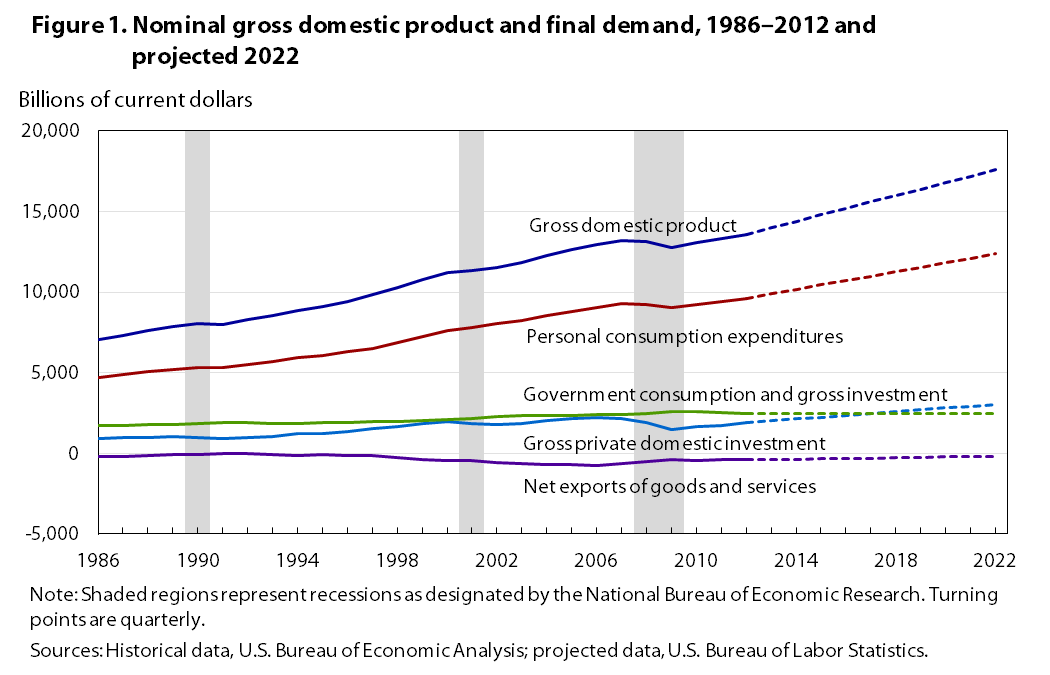
From 2012–2022, BLS expects GDP to grow at a rate of 2.6 percent per year, reaching $17.6 trillion in the target year of the projections. The unemployment rate is projected to gradually decrease to 5.4 percent, accompanied by a gain in household employment of 12.3 million jobs. Productivity growth is expected to remain strong at 2.0 percent per year, helping boost output growth, despite the expected slow growth in the labor force. Housing starts are estimated to average 1.6 million per year as construction accelerates, satisfying demand for new homes and replacements for aging structures. Export growth in excess of that of imports will help narrow the trade deficit, with real net exports equal to –179.1 billion in 2022.
The object of BLS macroeconomic projections is to develop a reasonable picture of the long-term economy that can be used as a framework for the Bureau’s more detailed industry output and employment projections. As such, the focus is on the long-run economic trends, not transitory economic phenomena, such as business cycle dynamics. Presented here are the primary assumptions made in the macro model, major trends for the decade encompassing 2012–2022, and an evaluation of uncertainty in the projections.
BLS macroeconomic projections are produced by using the MA/US model, licensed from Macroeconomic Advisers (MA), LLC.6 The 2012–2022 projections are the first to employ the new model, which was introduced in late 2012; previously, the Bureau relied on MA’s Washington University Macro Model (WUMM). MA/US has the same foundations as WUMM: consumption follows a life-cycle model and investment is based on a neoclassical model. Foreign sector estimates rely on forecasts from Oxford Economics. However, many improvements were made; most notably, the model is explicitly designed to reach a full-employment solution in the target years. Within MA/US, a submodel calculates an estimate of potential output from the nonfarm business sector, based upon full-employment7 estimates of the sector’s hours worked and output per hour. Error correction models are embedded into MA/US to align the model’s solution with the full-employment submodel.
Certain critical variables set the parameters for the nation’s economic growth and determine in a large part the trend that GDP will follow. In developing the macroeconomic projections, BLS elects to externally determine these critical variables through research and modeling and then supplies them to the MA/US model as exogenous variables. Table 1 provides a list of key assumptions made in the model.
| Exogenous variables | Billions of chained 2005 dollars (unless otherwise noted) | Annual rate of change | |||||
|---|---|---|---|---|---|---|---|
| 1992 | 2002 | 2012 | 2022 | 1992–2002 | 2002–2012 | 2012–2022 | |
Monetary policy related: | |||||||
Federal funds rate (percent) | 3.5 | 1.7 | 0.1 | 4.6 | -7.2 | -21.9 | 41.8 |
Ninety-day Treasury bill rate (percent) | 3.5 | 1.6 | .1 | 4.4 | -7.4 | -25.5 | 48.1 |
Yields on 10-year Treasury notes (percent) | 7.0 | 4.6 | 1.8 | 5.3 | -4.1 | -9.0 | 11.3 |
Fiscal policy, tax related: | |||||||
Effective federal marginal tax rate on wages and salaries (percent) | 21.3 | 22.5 | 21.4 | 21.4 | .6 | -.5 | .0 |
Effective federal marginal tax rate on interest income (percent) | 22.0 | 24.5 | 23.0 | 25.0 | 1.1 | -.6 | .8 |
Effective federal marginal tax rate on dividend income (percent) | 25.1 | 28.0 | 22.5 | 28.0 | 1.1 | -2.1 | 2.2 |
Effective federal marginal tax rate on capital gains (percent) | 25.7 | 18.8 | 15.0 | 20.0 | -3.1 | -2.2 | 2.9 |
Maximum federal corporate rate (percent) | 34.0 | 35.0 | 35.0 | 35.0 | .3 | .0 | .0 |
Fiscal policy, government outlays related: | |||||||
Defense intermediate goods and services purchased | 160.0 | 182.7 | 259.1 | 171.8 | 1.3 | 3.6 | -4.0 |
Defense gross investment | 67.9 | 59.6 | 97.0 | 75.1 | -1.3 | 5.0 | -2.5 |
Nondefense Intermediate goods and services purchased | 72.9 | 94.5 | 127.7 | 90.2 | 2.6 | 3.1 | -3.4 |
Nondefense gross investment | 28.6 | 34.2 | 46.8 | 44.0 | 1.8 | 3.2 | -.6 |
Federal grants-in-aid, Medicaid and other (billions of current dollars) | 149.1 | 304.1 | 468.0 | 646.9 | 7.4 | 4.4 | 3.3 |
Federal transfer payments, Medicare (billions of current dollars) | 132.6 | 259.2 | 562.0 | 980.3 | 6.9 | 8.0 | 5.7 |
Energy related: | |||||||
Price of West Texas Intermediate crude oil (nominal dollars per barrel) | 20.6 | 26.1 | 94.2 | 129.2 | 2.4 | 13.7 | 3.2 |
Price of Brent crude oil (nominal dollars per barrel) | 19.3 | 24.9 | 111.7 | 131.5 | 2.6 | 16.2 | 1.6 |
Price of natural gas (nominal dollars per million Btu) | 1.8 | 2.7 | 2.6 | 5.3 | 4.3 | -.4 | 7.5 |
Domestic oil product | 2.6 | 2.1 | 2.4 | 3.5 | -2.2 | 1.2 | 3.9 |
Demographic related: | |||||||
Total population, including overseas Armed Forces (millions) | 256.9 | 287.9 | 315.0 | 339.2 | 1.1 | .9 | .7 |
Population ages 16 and older (millions) | 192.8 | 217.6 | 243.3 | 265.3 | 1.2 | 1.1 | .9 |
| Sources: Historical data, U.S. Federal Reserve Board, U.S. Bureau of Economic Analysis, U.S. Census Bureau; projected data, U.S. Bureau of Labor Statistics, U.S. Energy Information Administration, U.S. Census Bureau. | |||||||
Demographics and the labor force. Growth in the labor force is the primary constraint on economic growth. At the beginning of the BLS projections process, detailed projections for the labor force participation rates of 136 demographic groups are modeled in-house and combined with the U.S. Census Bureau’s midrange population projections.8 The resulting labor force levels and age composition affect many key outputs of the model, such as housing starts, prices, and savings rate.
Growth in the civilian noninstitutional population ages 16 and over will continue to slow over the next decade, increasing at a compound annual rate of 0.9 percent from 243.3 million individuals in 2012 to 265.3 million in 2022. The U.S. labor force participation rate peaked at 67.1 percent from 1997–2000 and then began to drift downward, falling by about 1.0 percent before the onset of the 2007 recession. As the recession took hold, the decline in the participation rate accelerated, reaching 63.0 percent in November 2013, the most recent data available at the time of publication. As more of the baby-boom generation moves into retirement, the labor force participation rate is projected to decline another 1.4 percentage points by 2022, dropping to 61.6 percent. Coupled with the slowing population growth, the participation declines translate into slow growth of the labor force. From 2012–2022, the labor force is expected to grow from 155.0 million people to 163.5 million, an annual rate of 0.5 percent.
The nonaccelerating inflation rate of unemployment. The objective of the BLS projections is to provide a reasonable outlook on the nation’s potential economic future. Fluctuations in the business cycle are short term and hard to foresee, particularly on a 10-year horizon. Therefore, the projections are made by assuming a full-employment economy in the target year. In constructing such a scenario, a value for the nonaccelerating inflation rate of unemployment (NAIRU) needs to be supplied to the model. BLS estimate of the NAIRU is based on an assessment of historical trends and an extensive literature review. Although unemployment has remained high in the wake of the 2007–2009 recession, the forces keeping it elevated are expected to abate over time. Temporary elevations could be attributed to several factors, including structural changes leading to increased skills mismatch in the labor force, extensions of unemployment benefits, general uncertainty in the current economic climate, and a cyclical lack of demand for labor. By 2022, the unemployment rate is projected to equal the NAIRU, at 5.4 percent.
Fiscal and monetary policy. In recent years, fiscal policy in the United States has transitioned from expansionary to contractionary. During the recession, large-scale spending programs designed to stimulate the economy, primarily the American Recovery and Reinvestment Act of 2009 (ARRA), led to record budget deficits and sharp increases in the national debt. In response, measures to cut federal budgets were laid out in the Budget Control Act of 2011 (BCA), the stipulations of which specified that if lawmakers could not agree to a plan to reduce federal deficits over the coming decade, automatic spending cuts would go into effect across the board. These cuts have been popularly referred to as “the sequester.” After being postponed by the American Taxpayer Relief Act of 2012, the sequester went into effect in March 2013, enforcing cuts in both mandatory and discretionary spending. These cuts will cause a large decrease in outlays in the initial projection years, but spending is anticipated to accelerate in the latter years of the projection period to meet the needs of the nation’s aging population and fund the expansions to health insurance programs offered under the Patient Protection and Affordable Care Act.9 Without further reductions in outlays or increases in revenue, federal deficits would climb again, rapidly adding to the national debt and thereby maintaining the debt-to-GDP ratio at historically high levels. The MA/US model incorporates the cuts mandated by the BCA and assumes that spending restraint sufficient to keep the national debt at a manageable level will be exercised.
In response to the weak economy, the Federal Reserve has held interest rates at the lower bound since December 2008. In addition, the Federal Reserve has employed less traditional monetary policy. Three rounds of large-scale asset purchases were pursued, the last of which is currently anticipated to finish in mid-2014.10 Beginning December 2012, the Federal Open Market Committee began issuing explicit forward guidance outlining their expectations as to when a hike in the federal funds rate would occur and which levels of unemployment and inflation would likely trigger such a hike.11 Monetary policy is determined endogenously in the MA/US model through a vector autoregression (VAR). The VAR is designed to estimate the federal funds rate for each period according to the Federal Reserve’s dual mandate of maximizing employment while controlling inflation. For each period the model is run, the VAR forecasts the expected funds rate over 2- and 10-year horizons, ensuring that the resulting estimates are consistent with the model results as a whole.
Energy prices. The introduction of MA/US incorporated a greater variety of energy prices. Previously, only one measure of imported oil costs was included within the model; with the 2012–2022 projections, nominal prices for West Texas Intermediate (WTI) crude, Brent crude, and natural gas were used. All energy price projections come from the Energy Information Agency (EIA) Annual Energy Outlook (AEO) 2013.12 The AEO takes a long-run look at fuel production and consumption and incorporates the assumption that current energy regulations will remain unchanged. Because of advances in technology and increased fuel prices that make accessing previously unprofitable oil reserves possible, EIA anticipates that domestic oil production will rise, peaking in 2019. The nominal price of WTI is expected to increase from $94.20 per barrel in 2012 to $129.16 per barrel in 2022, while Brent crude is expected to increase from $111.74 per barrel in 2012 to $131.55 per barrel in 2022. Simultaneously, the burgeoning natural gas industry continues to benefit from increasing shale gas extractions, with the United States becoming a net exporter of natural gas by 2020 when domestic production is expected to outpace consumption. Nominal natural gas prices are expected to grow from $2.58 per million British thermal units (Btu) in 2012 to $5.35 per million Btu in 2022, a compound annual rate of 7.5 percent.
In 2012, the U.S. economy was still struggling to achieve the more rapid economic growth rates experienced prior to the 2007–2009 recession. Weak demand and economic uncertainty at home and abroad led firms to delay hiring and investment decisions, contributing to a still-elevated unemployment rate. Difficulty finding jobs, personal deleveraging, and tight credit conditions have in turn led to a slowdown in consumption. As the economy continues to struggle to return to potential growth levels, the nation finds itself facing a demographic shift and continued debt troubles. As the population ages, more workers leave the labor force and change their consumption habits accordingly, reducing consumer demand and investment in housing.13 An older population also draws more on social resources, driving entitlement spending up. The public sector will be forced to balance the increasing requirements of the citizens with the need to stabilize the debt-to-GDP ratio. With the slow labor force growth expected over the next decade, the economy will be less able to generate sustained periods of high growth. Instead, rates of progress that are more modest will become standard.
Evidence of the impact of the demographic shift on growth rates can be seen when one examines the first half of the prior decade, the 5 years preceding the 2007–2009 recession. Overall, GDP is expected to grow at 2.6 percent per year over the coming decade. (See table 2.) This growth is slower than the 3.4 percent annual growth experienced from 1992–2002 and slightly less than the prerecession growth rate of 2.7 percent annually seen from 2002–2007. Per capita GDP will increase at a rate of 1.9 percent per year, slightly faster than the 1.8 percent annual increase seen from 2002–2007 but slower than the 2.2 percent annual growth that occurred from 1992–2002.
| Category | Billions of chained 2005 dollars | Annual rate of change | Contribution to percent change in real GDP | |||||||
|---|---|---|---|---|---|---|---|---|---|---|
| 1992 | 2002 | 2012 | 2022 | 1992–2002 | 2002–2012 | 2012–2022 | 1992–2002 | 2002–2012 | 2012–2022 | |
Gross domestic product | $8,280.0 | $11,543.2 | $13,593.3 | $17,584.2 | 3.4 | 1.6 | 2.6 | 3.4 | 1.6 | 2.6 |
Personal consumption expenditures | 5,503.2 | 8,018.3 | 9,603.3 | 12,380.1 | 3.8 | 1.8 | 2.6 | 2.5 | 1.3 | 1.8 |
Gross private domestic investment | 983.1 | 1,800.4 | 1,914.4 | 3,038.2 | 6.2 | .6 | 4.7 | 1.0 | .1 | .7 |
Exports | 683.5 | 1,098.4 | 1,837.4 | 3,117.7 | 4.9 | 5.3 | 5.4 | .5 | .5 | .8 |
Imports(1) | 718.7 | 1,646.8 | 2,238.1 | 3,296.8 | 8.6 | 3.1 | 3.9 | -1.0 | -.5 | -.7 |
Government consumption expenditures and gross investment | 1,893.2 | 2,279.7 | 2,481.1 | 2,487.0 | 1.9 | .9 | .0 | .3 | .2 | .0 |
Federal defense | 549.8 | 505.3 | 677.2 | 560.0 | -.8 | 3.0 | -1.9 | -.1 | .2 | -.1 |
Federal nondefense | 233.3 | 274.0 | 347.1 | 302.1 | 1.6 | 2.4 | -1.4 | .0 | .1 | .0 |
State and local | 1,107.6 | 1,500.7 | 1,461.7 | 1,615.1 | 3.1 | -.3 | 1.0 | .3 | .0 | .1 |
Residual(2) | -61.8 | -6.9 | -9.7 | -132.1 | — | — | — | — | — | — |
Addenda: | ||||||||||
GDP per capita, chained 2005 dollars | 32,226.7 | 40,090.9 | 43,152.3 | 51,834.7 | 2.2 | .7 | 1.9 | — | — | — |
Notes: (2) The residual is calculated as real GDP, plus imports, less other components. Note: Dash indicates data not computable or not applicable. Sources: Historical data, U.S. Bureau of Economic Analysis, projected data, U.S. Bureau of Labor Statistics. | ||||||||||
Personal consumption expenditures. The largest component of demand is personal consumption expenditures (PCE), which compose approximately 70 percent of nominal GDP of the United States. (See table 3.) PCE exhibited robust growth of 3.8 percent annually from 1992–2002 and 2.9 percent annually from 2002–2007, facilitated by a declining personal savings rate and strong economic growth, which bolstered consumer confidence. Rapid increases in home prices characteristic of the housing bubble also contributed to the virtuous cycle of spending, while homeowners perceived an increase in their home equity. Because of the credit crisis and 2007–2009 recession, growth in consumption slowed dramatically to 0.7 percent per year over the second half of the decade. Hesitant to spend when faced with job insecurity, declining home values, and volatile stock prices, consumers reacted to the downturn by increasing their savings and reducing personal debt. Further, stricter lending standards reduced consumers’ access to credit, limiting their ability to spend as rapidly as in the past. From 2012 to 2022, PCE are expected to grow at the same rate as the economy as a whole, 2.6 percent annually.
| Category | Billions of dollars | Percent distribution | ||||||
|---|---|---|---|---|---|---|---|---|
| 1992 | 2002 | 2012 | 2022 | 1992 | 2002 | 2012 | 2022 | |
Gross domestic product | $6,342.3 | $10,642.3 | $15,684.8 | $24,144.1 | 100.0 | 100.0 | 100.0 | 100.0 |
Personal consumption expenditures | 4,236.9 | 7,439.2 | 11,119.6 | 17,025.0 | 66.8 | 69.9 | 70.9 | 70.5 |
Gross private domestic investment | 864.8 | 1,646.9 | 2,062.3 | 3,742.0 | 13.6 | 15.5 | 13.1 | 15.5 |
Exports | 635.0 | 1,003.0 | 2,184.1 | 4,069.6 | 10.0 | 9.4 | 13.9 | 16.9 |
Imports(1) | 667.8 | 1,430.2 | 2,744.0 | 4,695.9 | 10.5 | 13.4 | 17.5 | 19.4 |
Government consumption expenditures and gross investment | 1,273.4 | 1,983.3 | 3,062.8 | 4,003.4 | 20.1 | 18.6 | 19.5 | 16.6 |
Federal defense | 376.8 | 437.7 | 809.2 | 833.1 | 5.9 | 4.1 | 5.2 | 3.5 |
Federal nondefense | 156.1 | 243.0 | 405.1 | 428.8 | 2.5 | 2.3 | 2.6 | 1.8 |
State and local | 740.6 | 1,302.7 | 1,848.5 | 2,741.5 | 11.7 | 12.2 | 11.8 | 11.4 |
Notes: Sources: Historical data, U.S. Bureau of Economic Analysis, projected data, U.S. Bureau of Labor Statistics. | ||||||||
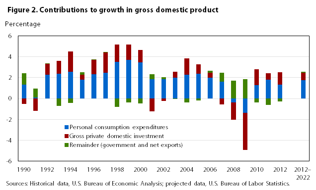
Of the 2.6 percentage points GDP is anticipated to gain per year, PCE are expected to contribute 1.8 points, or 67.4 percent of all economic growth. (See table 2 and figure 1.) This rate is a substantial slowdown from the previous decade, in which PCE made up 80.8 percent of all growth, and from the period 1992–2002, when PCE accounted for 75.3 percent of economic activity. Such a distributional change is usual following a recession, when resurgences in investment make the remaining components of GDP appear to be of lesser importance. (See figure 2.)
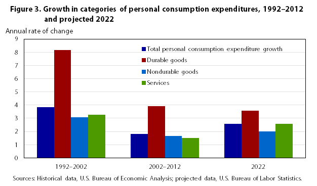
PCE can be divided into three categories: durable goods, nondurable goods, and services. The fastest growing segment is spending on durable goods, those purchases with a lifespan of 3 or more years, with an expected growth rate of 3.6 percent annually over the coming decade. (See figure 3 and table 4.) Durable goods tend to be expensive items, such as appliances, furniture, and televisions, the purchase of which consumers often elect to delay during an economic downturn. Indeed, consumption of durables grew at a rate of 8.2 percent per year from 1992–2002, 5.8 percent from 2002–2007, but dropped to 2.0 percent from 2007–2012. As the business cycle turns upward and consumers decide to reenter the market for durable goods, their contributions will be counteracted by the movement of the baby-boom generation into older age cohorts, whose changing needs redirect their spending into other sectors.
| Category | Billions of chained 2005 dollars | Annual rate of change | |||||
|---|---|---|---|---|---|---|---|
| 1992 | 2002 | 2012 | 2022 | 1992–2002 | 2002–2012 | 2012–2022 | |
Personal consumption expenditures | $5,503.2 | $8,018.3 | $9,603.3 | $12,380.1 | 3.8 | 1.8 | 2.6 |
Durable goods | 423.1 | 927.9 | 1,361.0 | 1,935.7 | 8.2 | 3.9 | 3.6 |
Motor vehicles and parts | 231.5 | 394.0 | 373.3 | 523.3 | 5.5 | -.5 | 3.4 |
Other durable goods | 205.5 | 536.2 | 995.5 | 1,439.0 | 10.1 | 6.4 | 3.8 |
Nondurable goods | 1,316.8 | 1,780.1 | 2,094.5 | 2,556.6 | 3.1 | 1.6 | 2.0 |
Food | 526.5 | 608.9 | 685.8 | 766.2 | 1.5 | 1.2 | 1.1 |
Gasoline | 249.1 | 294.0 | 268.6 | 287.6 | 1.7 | -.9 | .7 |
Other nondurable goods | 566.3 | 880.8 | 1,154.9 | 1,544.2 | 4.5 | 2.7 | 2.9 |
Services | 3,861.6 | 5,318.5 | 6,176.6 | 7,973.1 | 3.3 | 1.5 | 2.6 |
Housing services | 1,129.7 | 1,461.9 | 1,677.7 | 2,060.6 | 2.6 | 1.4 | 2.1 |
Imputed rent | 678.0 | 933.5 | 1,084.3 | 1,365.3 | 3.3 | 1.5 | 2.3 |
Natural gas | 63.5 | 61.2 | 57.4 | 63.2 | -.4 | -.6 | 1.0 |
Electricity | 93.1 | 118.6 | 126.6 | 160.7 | 2.4 | .7 | 2.4 |
Other housing services | 299.5 | 348.9 | 408.6 | 471.1 | 1.5 | 1.6 | 1.4 |
Medical services | 916.5 | 1,202.5 | 1,516.8 | 2,071.3 | 2.8 | 2.3 | 3.2 |
Other services | 1,819.0 | 2,654.1 | 2,980.8 | 3,833.9 | 3.9 | 1.2 | 2.5 |
Residual(1) | -145.4 | -14.6 | -49.3 | -145.8 | — | — | — |
Notes: Note: Dash indicates data not computable or not applicable. Sources: Historical data, U.S. Bureau of Economic Analysis, projected data, U.S. Bureau of Labor Statistics. | |||||||
Durable goods expenditures are classified as either purchases of motor vehicles and parts or other durable goods. Motor vehicles sales were particularly hard hit by the recession; increases in automobile reliability allowed cautious consumers to continue driving their older vehicles rather than replacing them with newer models.14 The number of units sold reached a trough of 10.4 million per year in 2009, down from a high of 16.9 in 2004 and 2005. The dramatic decline in sales resulted in consolidation and restructuring in the industry, and by 2012, sales had reached 14.4 million units. Sales of new automobiles are expected to average 14.8 million units per year over the coming decade, with higher volume in the earlier years of the projections period reflecting the conflicting pressures of pent-up demand and decreasing durable goods consumption of the elderly. With somewhat tighter lending standards than before the recession and increasing automobile lifespans, demand for new vehicles will be dampened. Total growth in consumption of motor vehicles and parts declined by 0.5 percent annually from 2002–2012, but it is expected to resume a healthy growth rate of 3.4 percent per year from 2012–2022.
The category of other durable goods is expected to reflect this conflict even more sharply. Growth in this category slowed from 10.1 percent annually from 1992–2002 to 6.4 percent annually for the period from 2002–2012 and is projected to slow even more, decreasing to 3.8 percent annually from 2012– 2022. This decline is largely attributable to consumers devoting a growing proportion of their income to nondurable goods and services. Within durable goods, digital devices continue to drive growth. The sectors that comprise the sales of televisions, personal computers, tablets, and smart phones are expected to grow at a pace that exceeds their historical trends. Sales of books, a comparatively small component of demand, will grow below trend, further reflecting a shift toward digital media.
Nondurable goods include many “essentials” for life, including food, medicines, clothing, and gasoline. The necessity of these items makes delaying or reducing spending in this category more difficult. Therefore, nondurable consumption has been somewhat more stable. Growth was 3.1 percent annually from 1992–2002 and declined to 1.6 percent annually for the period from 2002–2012. Growth is expected to remain steady at a rate of 2.0 percent annually over the projections period. The recession slightly affected spending on food, with the annual rate from 2002–2012 equal to 1.2 percent, compared with the 1.5 percent annual growth seen from 1992–2002. Growth over the next decade is expected to slow to 1.1 percent per year, as consumers make choices that are more careful and apportion more of their incomes to health needs. Gasoline expenditures fell at a rate of 0.9 percent per year from 2002–2012, largely because of rapid increases in petroleum prices and deteriorating economic conditions in the latter half of the decade. Consumption of gasoline is expected to rise again over the next 10 years, although it will be kept in check by continued rises in oil prices and shifts to renewable energy and more fuel-efficient technologies. Gasoline expenditures are forecast to continue to increase at a modest pace of 0.7 percent per year to 2022.
Services are the largest component of PCE; its share of nominal consumer spending grew steadily from 64.9 percent in 1992 to 66.0 percent in 2012 and is expected to constitute 70.2 percent by 2022. Services increased at a rate of 3.3 percent annually from 1992–2002, declining to 1.5 percent from 2002–2012, but the effects on the various categories of services were disparate, as are their paths going forward. Housing services was sharply affected, falling to an annual growth rate of 0.6 percent from 2007–2012 from a rate of 2.2 percent from 2002–2007, and 2.6 percent from 1992 through 2002. This category is largely composed of imputed rent, the estimate of what an owner-occupier would have paid in rent had they been leasing the home. With the large declines in home prices after the housing bubble burst, growth of imputed rents stalled. As home prices increase, growth in the consumption of housing services is expected to return to the prerecession trend, with a projected annual growth rate through 2022 of 2.1 percent. Medical services remained steady over the prior decade, exhibiting growth rates of 2.3 percent per year, compared with the 2.8 percent annually seen from 1992–2002. With the expansion of health insurance under the Patient Protection and Affordable Care Act, advances in medical technologies, and increasing demand from the aging population, consumption of medical services is expected to grow faster over the projections horizon at a rate of 3.2 percent per year. The grouping of “other services” includes categories of spending such as personal care and telecommunications. Like durable goods, “other services” is an area in which consumers can more easily cut back their spending. Growth in other services fell from 3.9 percent annually from 1992–2002 to 1.2 percent for the decade from 2002–2012 and is expected to remain slow, growing at 2.5 percent annually until 2022.
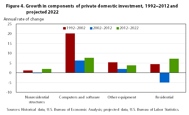
Residential investment. Growth in residential investment has been a key component of prior economic recoveries in the United States. Population growth inherently creates demand for housing, which creates jobs in construction and has spillover effects in other sectors as a result of home buyers furnishing their new abodes. In the wake of the housing bubble of the mid-2000s, home prices remained depressed and strict lending standards prevented some consumers from accessing the market. High foreclosure rates flooded the market with an excess supply of homes, causing many to remain on the market for extended periods. First-time home-buyer tax credits were offered in 2008–2010 but did little to boost sales. Residential investment, which grew at 4.4 percent annually from 1992–2002, shrunk at a rate of 5.0 percent per year from 2002–2012. (See figure 4 and table 5.) Single-family homes were particularly hard hit, decreasing 8.9 percent per year over the past decade, compared with multifamily units, which fell at a rate of 7.8 percent per year.
| Category | Billions of chained 2005 dollars | Annual rate of change | |||||
|---|---|---|---|---|---|---|---|
| 1992 | 2002 | 2012 | 2022 | 1992–2002 | 2002–2012 | 2012–2022 | |
Gross private domestic investment | $983.1 | $1,800.4 | $1,914.4 | $3,038.2 | 6.2 | 0.6 | 4.7 |
Fixed nonresidential investment | 600.4 | 1,173.7 | 1,487.8 | 2,241.9 | 6.9 | 2.4 | 4.2 |
Equipment and software | 347.2 | 824.2 | 1,143.9 | 1,868.2 | 9.0 | 3.3 | 5.0 |
Computers and software | 36.9 | 231.2 | 425.8 | 888.1 | 20.1 | 6.3 | 7.6 |
Other equipment | 352.1 | 595.0 | 725.5 | 1,048.2 | 5.4 | 2.0 | 3.7 |
Structures | 317.9 | 356.6 | 353.6 | 431.5 | 1.2 | -.1 | 2.0 |
Fixed residential structures | 397.3 | 613.8 | 367.1 | 733.8 | 4.4 | -5.0 | 7.2 |
Single family | 218.3 | 327.6 | 128.9 | 405.5 | 4.1 | -8.9 | 12.1 |
Multifamily | 21.9 | 38.9 | 17.2 | 41.6 | 5.9 | -7.8 | 9.2 |
Other | 156.6 | 246.9 | 223.1 | 294.4 | 4.7 | -1.0 | 2.8 |
Change in business inventories | 17.9 | 12.8 | 43.0 | 45.4 | -3.3 | 12.9 | .6 |
Residual(1) | -138.6 | -8.6 | -2.8 | -116.6 | — | — | — |
Notes: Note: Dash indicates data not computable or not applicable. Sources: Historical data, U.S. Bureau of Economic Analysis, projected data, U.S. Bureau of Labor Statistics. | |||||||
In recent months, evidence of the long-awaited housing recovery has emerged.15 Multifamily starts are back to the prerecessionary levels, and inventories of single-family homes are decreasing, causing home prices to rise. There is still reason to believe that a stronger housing recovery remains on the horizon. Household formation rates, which respond to business cycle dynamics, have been low in recent years, creating the potential for a sizable boost to the market as individuals regain economic confidence.16 Fundamentally, the housing market is demographically driven, and new construction will be needed to house the growing population and replace aging structures. Over the coming decade, BLS expects that total residential investment will increase 7.2 percent per year, with single-family home starts growing at a rate of 12.1 percent annually and multifamily construction growing 9.2 percent annually. Housing starts will average 1.6 million per year over the decade.
Nonresidential investment. The last 10 years were particularly tumultuous for nonresidential investment. Coming off a decade of robust growth at 6.9 percent annually in the 1990s, investment suffered after the dot-com bubble burst, contributing to the recession that lasted from March to November 2001. Still, growth gradually increased, reaching 5.7 percent annual growth for the 5 years preceding the 2007–2009 recession. The recession severely limited the willingness and ability of businesses to invest in new equipment and structures. From 2007–2012, this demand component shrank at a rate of 0.8 percent per year. Over the coming decade, nonresidential investment as a whole is expected to grow at a rate of 4.2 percent.
Investment in computers and software was the only category of fixed investment that did not decline throughout the recession and recovery. Though far short of the 20.1 percent annual growth seen from 1992–2002, computers and software investment gained 6.3 percent annually over the last decade, including growth of 4.0 percent per year from 2007–2012. This growth was fed by the increased automation and network building. Robust growth, though moderate by some historical standards, is anticipated at 7.6 percent per year through 2022. Investment in nonresidential structures, which includes factories, medical facilities, schools, and offices, experienced declines that were more noticeable during the recession. These structures have long service lives, and as such, construction is based upon long-run growth forecasts.17 Strong economic performance in the mid-2000s and optimism about the future led to the rapid construction, which in turn led to an excess of structures when the recession hit. After growing at 4.2 percent annually from 2002–2007, trends were reversed, with net growth over the decade equal to –0.1 percent annually. Because of the long lifespan of these structures, the excess supply takes particularly long to absorb as compared with other forms of investment. Going forward, nonresidential structures are expected to grow at 2.0 percent annually, gaining momentum in the latter years of the projections period.
Foreign trade in goods and services and the current account. Foreign trade represents an area of considerable uncertainty in the macroeconomic projections, especially because of the global nature of the recent economic slowdown. As nations recover at different rates or experience other crises, the precise path of global trade is difficult to anticipate, although generally the sector will be of ever-growing importance. The past two decades have seen a rapid increase in globalization, with rising volumes of both imports into and exports out of the United States. Increasing integration has acted as a double-edged sword, bringing Americans access to cheaper goods from overseas, while simultaneously leading to the offshoring of many labor-intensive industries. The accession of China to the World Trade Organization in 2001 was milestone in the progression of globalization, opening new arenas for investment while dramatically increasing the availability of Chinese exports in world markets. Going forward, the United States can expect to be increasingly affected by changes in foreign economies. Gradual factor price equalization will limit the gains firms can achieve by outsourcing production. The anticipated slowdown of growth in China and other emerging markets can potentially limit imports to the United States.18 Many of the structural changes that globalization brought to the nation are expected to persist. The United States has long had a positive balance of trade for services and a substantial trade deficit for goods, both of which are expected to continue as the U.S. economy remains largely service based.
During the decade leading up to the 2007–2009 recession, the trade deficit deepened considerably. Net exports grew at an annual rate of 20.8 percent, widening the trade deficit to $729.4 billion in 2006. As economies worldwide felt the effects of the financial crisis, both imports and exports slowed, though imports fell faster than exports, leading to a narrowing of the trade deficit. This tightening is expected to continue, with the real trade deficit shrinking from $400.7 billion in 2012 to $179.1 billion in 2022, while the personal savings rate stabilizes and federal deficits decline. (See table 6.) Export growth is expected to be slightly faster than the historical trend of the last two decades, while imports grow more slowly.
| Category | Billions of chained 2005 dollars | Annual rate of change | |||||
|---|---|---|---|---|---|---|---|
| 1992 | 2002 | 2012 | 2022 | 1992–2002 | 2002–2012 | 2012–2022 | |
Exports of goods and services | $683.5 | $1,098.4 | $1,837.4 | $3,117.7 | 4.9 | 5.3 | 5.4 |
Goods | 454.2 | 762.7 | 1,300.4 | 2,231.5 | 5.3 | 5.5 | 5.5 |
Nonagricultural | 401.7 | 698.1 | 1,215.8 | 2,138.5 | 5.7 | 5.7 | 5.8 |
Agricultural | 52.6 | 64.4 | 86.5 | 115.2 | 2.0 | 3.0 | 2.9 |
Services | 233.4 | 335.6 | 537.5 | 889.9 | 3.7 | 4.8 | 5.2 |
Residual(1) | -4.2 | .3 | -2.5 | -25.9 | — | — | — |
Imports of goods and services | 718.7 | 1,646.8 | 2,238.1 | 3,296.8 | 8.6 | 3.1 | 3.9 |
Goods | 563.1 | 1,372.2 | 1,858.2 | 2,786.2 | 9.3 | 3.1 | 4.1 |
Nonpetroleum | 456.6 | 1,157.6 | 1,687.9 | 2,732.2 | 9.8 | 3.8 | 4.9 |
Petroleum | 146.4 | 217.1 | 204.9 | 197.5 | 4.0 | -.6 | -.4 |
Services | 162.4 | 274.5 | 381.9 | 514.3 | 5.4 | 3.4 | 3.0 |
Residual(2) | -46.7 | -2.4 | -36.7 | -147.2 | — | — | — |
Trade surplus/deficit | -35.2 | -548.5 | -400.7 | -179.1 | 31.6 | -3.1 | -7.7 |
Notes: (2) The residual is the difference between the aggregate for “imports of goods and services” and its detailed components. Note: Dash indicates data not computable or not applicable. Sources: Historical data, U.S. Bureau of Economic Analysis, projected data, U.S. Bureau of Labor Statistics. | |||||||
The current account balance (CAB) measures income flows into and out of the United States, in addition to net exports. The CAB has widened substantially since the 1990s, because the trade deficit grew and income payments to the rest of the world increased. The current account deficit, measured in nominal terms, grew to be $798.4 billion in 2006, before retreating during the recession. Continued rebalancing is expected through 2022, with the CAB projected to decline from $474.1 billion to $63.2 billion from 2012–2022. Income receipts from the rest of the world are projected to outpace income payments, in part, because of a differential rate of return on investments abroad. As a percentage of nominal GDP, the CAB is expected to be only 0.3 percent in 2022, down from 3.0 percent in 2012.
As a strong and stable economy, the United States is seen as a desirable destination for foreign investment, which facilitated the steep rise in the broad trade-weighted exchange rate for the U.S. dollar from the mid-1980s to the early 2000s. With pressure from the nation’s increasing trade deficits and recessions in 2001 and 2007–2009, downward pressure was exerted on the dollar and the exchange rate declined by more than 20 percent from 2002–2012. Going forward, the exchange rate is expected to remain relatively stable. The United States currently presents a more sound investment possibility than the European Union (EU), which is still dealing with the aftermath of several nations’ sovereign debt crises, while emerging markets provide increased competition for foreign dollars. The anticipated narrowing of the trade deficit will also alleviate pressure on the dollar. On balance, the forces will counteract each other and the expected result is a modest 4.1 percent increase in the exchange rate by 2022.
Federal government. In the coming years, the federal government will be subjected to two major, conflicting pressures: the need to meet the demands of the aging population while simultaneously stabilizing the debt-to-GDP ratio.19 In an attempt to stimulate the economy in the wake of the 2007–2009 recession, massive spending programs were enacted, including the American Recovery and Reinvestment Act, the Troubled Asset Relief Program, bailouts for the automobile industry, and the government takeover of Fannie Mae and Freddie Mac. Coupled with low revenues stemming from the sluggish economy and extensions to the Bush-era tax cuts, federal deficits rose rapidly, with shortfalls in excess of $1 trillion for each year from 2009–2012.20 Such large deficits rapidly added to the national debt, bringing the value of the debt held by the public to 72.5 percent of GDP at the end of 2012, the highest level seen since World War II. A sustained high level of debt-to-GDP ratio can damage economic growth because it makes investors less willing to lend to the U.S. government and risks sparking a financial crisis. Higher debts also come with increased interest payments, further adding to the government’s fiscal dilemma and hampering the future flexibility of policies in the face of further economic adversity. After the sequester reduced federal government spending, federal agencies implemented the spending cuts in a variety of ways, including eliminating programs and furloughing employees. When the data presented here were finalized for publication, impacts of the sequester were only beginning to be seen in economic data. Research shows that the contractionary policies of the federal government may restrain GDP growth as much as 1 percentage point per year over the next 3 years.21
As the baby-boom generation reaches retirement age, outlays for entitlement programs will increase substantially. (See table 7.) More individuals will become eligible for Social Security and Medicare, and as individuals live longer and medical technologies increase, so will healthcare spending. In addition, the passage of the Patient Protection and Affordable Care Act in 2010 will gradually expand health insurance coverage to millions of citizens, in part through large federal subsidies. These dramatic increases to nondiscretionary spending are directly at odds with the aforementioned need to control federal deficits. As a result, mandatory spending is expected to crowd out spending on other programs. The Congressional Budget Office estimates that even after sequestration, under current laws, deficits will begin to rise again by 2017 because of these programs. As discussed earlier, assumptions within the MA/US model include spending cuts that go beyond those mandated by the sequester, implying that further action will be taken to control spending. Even with these additional measures, BLS projects that the national debt will remain greater than 70 percent of GDP by the end of 2022.
| Category | Billions of current dollars | Percent distribution | Annual rate of change | ||||||||
|---|---|---|---|---|---|---|---|---|---|---|---|
| 1992 | 2002 | 2012 | 2022 | 1992 | 2002 | 2012 | 2022 | 1992–2002 | 2002–2012 | 2012–2022 | |
Receipts | $1,148.0 | $1,859.3 | $2,675.7 | $4,453.1 | 100.0 | 100.0 | 100.0 | 100.0 | 4.9 | 3.7 | 5.2 |
Tax receipts | 660.0 | 1,073.5 | 1,645.5 | 2,652.8 | 57.5 | 57.7 | 61.5 | 59.6 | 5.0 | 4.4 | 4.9 |
Personal taxes | 475.3 | 828.6 | 1,140.0 | 2,106.3 | 41.4 | 44.6 | 42.6 | 47.3 | 5.7 | 3.2 | 6.3 |
Corporate income taxes | 118.8 | 150.4 | 372.3 | 357.0 | 10.3 | 8.1 | 13.9 | 8.0 | 2.4 | 9.5 | -.4 |
Taxes on production and imports | 63.3 | 86.8 | 116.0 | 165.6 | 5.5 | 4.7 | 4.3 | 3.7 | 3.2 | 2.9 | 3.6 |
Taxes from the rest of the world | 2.7 | 7.6 | 17.3 | 23.8 | .2 | .4 | .6 | .5 | 11.1 | 8.6 | 3.2 |
Contributions for social insurance | 444.0 | 739.3 | 935.5 | 1,650.7 | 38.7 | 39.8 | 35.0 | 37.1 | 5.2 | 2.4 | 5.8 |
Income receipts on assets | 24.8 | 20.2 | 32.6 | 39.2 | 2.2 | 1.1 | 1.2 | .9 | -2.0 | 4.9 | 1.9 |
Interest receipts | 22.3 | 15.4 | 25.7 | 28.9 | 1.9 | .8 | 1.0 | .6 | -3.6 | 5.3 | 1.2 |
Rents and royalties | 2.5 | 4.8 | 6.9 | 10.3 | .2 | .3 | .3 | .2 | 6.7 | 3.6 | 4.1 |
Transfer receipts | 19.3 | 26.1 | 59.0 | 92.5 | 1.7 | 1.4 | 2.2 | 2.1 | 3.0 | 8.5 | 4.6 |
From business | 15.3 | 15.4 | 38.7 | 65.0 | 1.3 | .8 | 1.4 | 1.5 | .1 | 9.7 | 5.3 |
From persons | 4.1 | 10.8 | 20.3 | 27.5 | .4 | .6 | .8 | .6 | 10.1 | 6.6 | 3.1 |
Surplus of government enterprises | -.1 | .2 | -17.7 | -3.0 | .0 | .0 | -.7 | -.1 | — | — | -16.3 |
Expenditures | 1,450.5 | 2,112.1 | 3,757.7 | 5,314.2 | 100.0 | 100.0 | 100.0 | 100.0 | 3.8 | 5.9 | 3.5 |
Consumption expenditures | 444.1 | 590.5 | 1,059.7 | 1,126.9 | 30.6 | 28.0 | 28.2 | 21.2 | 2.9 | 6.0 | .6 |
Transfer payments | 725.4 | 1,252.1 | 2,319.1 | 3,438.9 | 50.0 | 59.3 | 61.7 | 64.7 | 5.6 | 6.4 | 4.0 |
Government social benefits | 555.7 | 924.6 | 1,792.8 | 2,703.3 | 38.3 | 43.8 | 47.7 | 50.9 | 5.2 | 6.8 | 4.2 |
Social Security benefits | 281.8 | 446.9 | 762.2 | 1,298.9 | 19.4 | 21.2 | 20.3 | 24.4 | 4.7 | 5.5 | 5.5 |
Medicare benefits | 132.6 | 259.2 | 562.0 | 980.3 | 9.1 | 12.3 | 15.0 | 18.4 | 6.9 | 8.0 | 5.7 |
Unemployment benefits | 39.6 | 53.5 | 80.9 | 35.0 | 2.7 | 2.5 | 2.2 | .7 | 3.0 | 4.2 | -8.0 |
Other benefits to persons | 95.5 | 155.3 | 369.9 | 365.1 | 6.6 | 7.4 | 9.8 | 6.9 | 5.0 | 9.1 | -.1 |
Benefits to the rest of the world | 6.2 | 9.6 | 17.9 | 23.9 | .4 | .5 | .5 | .5 | 4.5 | 6.3 | 3.0 |
Other transfer payments | 169.7 | 327.4 | 526.4 | 735.7 | 11.7 | 15.5 | 14.0 | 13.8 | 6.8 | 4.9 | 3.4 |
Grants-in-aid to state and local governments | 149.1 | 304.1 | 468.0 | 646.9 | 10.3 | 14.4 | 12.5 | 12.2 | 7.4 | 4.4 | 3.3 |
Transfer payments to the rest of the world | 20.5 | 23.3 | 58.3 | 88.7 | 1.4 | 1.1 | 1.6 | 1.7 | 1.3 | 9.6 | 4.3 |
Interest payments | 251.3 | 229.1 | 318.5 | 719.3 | 17.3 | 10.8 | 8.5 | 13.5 | -.9 | 3.4 | 8.5 |
To persons and business | 212.2 | 154.2 | 188.2 | 329.5 | 14.6 | 7.3 | 5.0 | 6.2 | -3.1 | 2.0 | 5.8 |
To the rest of the world | 39.1 | 74.9 | 130.4 | 389.9 | 2.7 | 3.5 | 3.5 | 7.3 | 6.7 | 5.7 | 11.6 |
Subsidies | 29.7 | 40.5 | 60.4 | 29.0 | 2.0 | 1.9 | 1.6 | .5 | 3.2 | 4.1 | -7.1 |
Less wage accruals less disbursements | .0 | .0 | .0 | .0 | — | — | — | — | — | — | — |
Net federal government saving | -302.5 | -252.8 | -1,082.0 | -861.1 | — | — | — | — | -1.8 | 15.7 | -2.3 |
Surplus or deficit as percentage of gross domestic product | -4.8 | -2.4 | -6.9 | -3.6 | — | — | — | — | -6.7 | 11.3 | -6.4 |
Note: Dash indicates data not computable or not applicable. Sources: Historical data, U.S. Bureau of Economic Analysis; projected data, U.S. Bureau of Labor Statistics. | |||||||||||
Defense spending was not exempt from the sequester. Coupled with the withdrawals of troops from Iraq and Afghanistan, this category represents an area of substantial decline in government spending. Defense consumption and investment grew at a rate of 3.0 percent annually from 2002–2012 but is expected to decrease at a rate of 1.9 percent annually through 2022. (See table 8.) Military personnel and healthcare costs and along with veterans’ benefits programs expanded considerably since 2001, representing a funding commitment over the next 40 years to provide for the well-being of servicemembers and their families.22 Furthermore, costs to replace equipment used in the wars in Iraq and Afghanistan and to maintain a presence in the region will be substantial. Because of such programs, a decreasing proportion of the defense budget will be available to fund core defense functions and fund research and development and a growing budget for the Department of Veterans Affairs will constrain the federal budget as a whole.
| Category | Billions of chained 2005 dollars | Annual rate of change | |||||
|---|---|---|---|---|---|---|---|
| 1992 | 2002 | 2012 | 2022 | 1992–2002 | 2002–2012 | 2012–2022 | |
Government consumption expenditures and gross investment | $1,893.2 | $2,279.7 | $2,481.1 | $2,487.0 | 1.9 | 0.9 | 0.0 |
Federal government consumption and investment | 783.0 | 779.5 | 1,024.1 | 861.6 | .0 | 2.8 | -1.7 |
Defense consumption and investment | 549.8 | 505.3 | 677.2 | 560.0 | -.8 | 3.0 | -1.9 |
Consumption expenditures | 479.7 | 445.8 | 580.5 | 484.1 | -.7 | 2.7 | -1.8 |
Compensation, military | 168.7 | 138.7 | 157.9 | 155.9 | -1.9 | 1.3 | -.1 |
Compensation, civilian | 95.4 | 65.1 | 81.4 | 78.0 | -3.7 | 2.3 | -.4 |
Consumption of fixed capital | 71.5 | 65.1 | 87.4 | 80.1 | -.9 | 3.0 | -.9 |
Intermediate goods and services purchased | 160.0 | 182.7 | 259.1 | 171.8 | 1.3 | 3.6 | -4.0 |
Less own-account investment | 2.8 | 2.5 | 1.9 | 1.7 | -1.0 | -2.6 | -1.2 |
Less sales to other sectors | 3.6 | 2.4 | 3.1 | 2.1 | -3.8 | 2.5 | -4.0 |
Gross investment | 67.9 | 59.6 | 97.0 | 75.1 | -1.3 | 5.0 | -2.5 |
Own-account investment | 2.8 | 2.5 | 1.9 | 1.7 | -1.0 | -2.6 | -1.2 |
Other investment | 65.3 | 57.2 | 95.1 | 73.4 | -1.3 | 5.2 | -2.6 |
Nondefense consumption and investment | 233.3 | 274.0 | 347.1 | 302.1 | 1.6 | 2.4 | -1.4 |
Consumption expenditures | 205.2 | 239.7 | 300.3 | 259.0 | 1.6 | 2.3 | -1.5 |
Compensation | 132.3 | 127.1 | 146.1 | 140.9 | -.4 | 1.4 | -.4 |
Consumption of fixed capital | 15.8 | 24.0 | 33.5 | 35.9 | 4.3 | 3.4 | .7 |
Commodity credit corporation purchases | -.7 | .1 | .0 | .0 | — | -6.7 | — |
Other intermediate goods and services purchased | 73.7 | 94.4 | 127.6 | 90.2 | 2.5 | 3.1 | -3.4 |
Less own-account investment | 4.3 | 2.7 | 2.5 | 2.8 | -4.5 | -.8 | 1.2 |
Less sales to other sectors | 7.3 | 3.1 | 4.5 | 5.0 | -8.3 | 3.9 | 1.1 |
Gross investment | 28.6 | 34.2 | 46.8 | 44.0 | 1.8 | 3.2 | -.6 |
Own-account investment | 4.3 | 2.7 | 2.5 | 2.8 | -4.5 | -.8 | 1.2 |
Other investment | 24.8 | 31.5 | 44.3 | 41.2 | 2.4 | 3.5 | -.7 |
State and local government consumption and investment | 1,107.6 | 1,500.7 | 1,461.7 | 1,615.1 | 3.1 | -.3 | 1.0 |
Consumption expenditures | 918.7 | 1,211.2 | 1,218.9 | 1,312.1 | 2.8 | .1 | .7 |
Compensation | 745.9 | 876.7 | 882.8 | 954.6 | 1.6 | .1 | .8 |
Consumption of fixed capital | 69.4 | 104.1 | 131.7 | 158.5 | 4.1 | 2.4 | 1.9 |
Intermediate goods and services purchased | 326.3 | 535.2 | 532.2 | 565.5 | 5.1 | -.1 | .6 |
Less own-account investment | 13.9 | 19.1 | 17.2 | 19.9 | 3.2 | -1.0 | 1.5 |
Less sales to other sectors | 203.7 | 285.3 | 310.4 | 345.1 | 3.4 | .8 | 1.1 |
Gross investment | 190.0 | 289.5 | 244.0 | 303.8 | 4.3 | -1.7 | 2.2 |
Own-account investment | 13.9 | 19.1 | 17.2 | 19.9 | 3.2 | -1.0 | 1.5 |
Other investment | 176.1 | 270.4 | 226.8 | 283.8 | 4.4 | -1.7 | 2.3 |
Residual(1) | -16.7 | -1.8 | -7.0 | 9.5 | — | — | — |
Notes: Note: Dash indicates data not computable or not applicable. Sources: Historical data, U.S. Bureau of Economic Analysis, projected data, U.S. Bureau of Labor Statistics. | |||||||
State and local governments. The vast majority of states have provisions that prevent them from running budget deficits, meaning that their fiscal decisions are forced to respond more rapidly to economic pressures. When incomes decline, states receive less in tax revenues while facing greater demand for social assistance programs, such as unemployment insurance and Medicaid. Cutbacks in federal grants further constrain state and local government spending. Compared with the decade from 1992–2002, every major category of state and local government expenditures experienced slower or negative growth from 2002–2012. (See table 9.) As a percentage of nominal expenditures, social benefits rose from 22.7 percent to 25.2 percent, while consumption expenditures decreased 1.9 percentage points to 69.6 percent, indicating that states were spending proportionally less on infrastructure projects, education, and other state-sponsored programs.
| Category | Billions of current dollars | Percent distribution | Annual rate of change | ||||||||
|---|---|---|---|---|---|---|---|---|---|---|---|
| 1992 | 2002 | 2012 | 2022 | 1992 | 2002 | 2012 | 2022 | 1992–2002 | 2002–2012 | 2012–2022 | |
Receipts | $846.2 | $1,412.7 | $2,069.5 | $3,315.2 | 100.0 | 100.0 | 100.0 | 100.0 | 5.3 | 3.9 | 4.8 |
Tax receipts | 579.8 | 928.7 | 1,398.0 | 2,371.0 | 68.5 | 65.7 | 67.5 | 71.5 | 4.8 | 4.2 | 5.4 |
Personal taxes | 135.3 | 221.8 | 335.8 | 565.9 | 16.0 | 15.7 | 16.2 | 17.1 | 5.1 | 4.2 | 5.4 |
Corporate income taxes | 24.4 | 30.9 | 48.2 | 106.7 | 2.9 | 2.2 | 2.3 | 3.2 | 2.4 | 4.6 | 8.3 |
Taxes on production and imports | 420.1 | 676.0 | 1,014.0 | 1,698.4 | 49.6 | 47.8 | 49.0 | 51.2 | 4.9 | 4.1 | 5.3 |
Sales taxes and other | 235.4 | 386.6 | 566.3 | 877.2 | 27.8 | 27.4 | 27.4 | 26.5 | 5.1 | 3.9 | 4.5 |
Property taxes | 184.7 | 289.4 | 447.7 | 821.1 | 21.8 | 20.5 | 21.6 | 24.8 | 4.6 | 4.5 | 6.3 |
Contributions for social insurance | 13.1 | 15.9 | 17.5 | 25.6 | 1.6 | 1.1 | .8 | .8 | 1.9 | .9 | 3.9 |
Income receipts on assets | 64.8 | 79.7 | 85.4 | 104.9 | 7.7 | 5.6 | 4.1 | 3.2 | 2.1 | .7 | 2.1 |
Interest receipts | 59.6 | 71.5 | 72.1 | 85.8 | 7.0 | 5.1 | 3.5 | 2.6 | 1.8 | .1 | 1.7 |
Dividends | .4 | 1.5 | 2.1 | 2.8 | .1 | .1 | .1 | .1 | 13.2 | 3.2 | 2.6 |
Rents and royalties | 4.8 | 6.6 | 11.2 | 16.4 | .6 | .5 | .5 | .5 | 3.3 | 5.4 | 3.9 |
Transfer receipts | 180.3 | 382.3 | 584.9 | 813.8 | 21.3 | 27.1 | 28.3 | 24.5 | 7.8 | 4.3 | 3.4 |
Federal grants-in-aid | 149.1 | 304.1 | 468.0 | 646.9 | 17.6 | 21.5 | 22.6 | 19.5 | 7.4 | 4.4 | 3.3 |
From business (net) | 9.3 | 32.5 | 45.7 | 71.1 | 1.1 | 2.3 | 2.2 | 2.1 | 13.4 | 3.4 | 4.5 |
From persons | 21.9 | 45.7 | 71.2 | 95.7 | 2.6 | 3.2 | 3.4 | 2.9 | 7.6 | 4.5 | 3.0 |
Surplus of government enterprises | 8.3 | 6.1 | -16.3 | .0 | 1.0 | .4 | -.8 | .0 | -3.0 | — | — |
Expenditures | 847.6 | 1,466.8 | 2,198.5 | 3,248.1 | 100.0 | 100.0 | 100.0 | 100.0 | 5.6 | 4.1 | 4.0 |
Consumption expenditures | 606.2 | 1,049.4 | 1,530.8 | 2,226.8 | 71.5 | 71.5 | 69.6 | 68.6 | 5.6 | 3.8 | 3.8 |
Government social benefit payments to persons | 180.0 | 333.0 | 554.2 | 852.4 | 21.2 | 22.7 | 25.2 | 26.2 | 6.3 | 5.2 | 4.4 |
Medicaid | 121.8 | 258.6 | 430.4 | 698.5 | 14.4 | 17.6 | 19.6 | 21.5 | 7.8 | 5.2 | 5.0 |
Other | 58.2 | 74.4 | 123.9 | 153.9 | 6.9 | 5.1 | 5.6 | 4.7 | 2.5 | 5.2 | 2.2 |
Interest payments | 61.0 | 83.5 | 113.0 | 168.3 | 7.2 | 5.7 | 5.1 | 5.2 | 3.2 | 3.1 | 4.1 |
Subsidies | .4 | .9 | .5 | .6 | .0 | .1 | .0 | .0 | 8.7 | -6.0 | 1.8 |
Less wage accruals less disbursements | .0 | .0 | .0 | .0 | .0 | .0 | .0 | .0 | — | — | — |
Net state and local government saving | -1.4 | -54.1 | -128.9 | 67.1 | — | — | — | — | — | — | — |
Note: Dash indicates data not computable or not applicable. Sources: Historical data, U.S. Bureau of Economic Analysis; projected data, U.S. Bureau of Labor Statistics. | |||||||||||
As the economy improves in the coming decade, state and local government receipts are expected to increase, gaining 4.8 percent annually from 2012–2022. Property taxes in particular will boost revenues as home prices rebound. As the federal government works to cut its spending, growth in grants is expected to slow to 3.3 percent annually from 2012–2022, compared with 4.4 percent annually in the prior decade. The expansion of Medicaid in some states as a part of the Patient Protection and Affordable Care Act will increase expenditures at the same time, making Medicaid payments 21.5 percent of total state and local expenditures, up from 17.6 percent in 2002 and 19.6 percent in 2012. This increase in spending will further crowd out other government programs, with other consumption decreasing to 68.6 percent of expenditures. Payments for social benefit programs other than Medicaid are expected to decrease to 4.7 percent of total expenditures, down from 5.6 percent, as fewer individuals qualify for unemployment insurance, food stamps, and other countercyclical spending programs.
On balance, total spending by governments will have a largely neutral impact on GDP over the coming decade. (See table 2.) Federal consumption and gross investment is anticipated to decline at a rate of 1.7 percent annually from 2012–2022, restraining GDP growth by a cumulative 0.1 percentage point over the period. Simultaneously, state and local consumption and investment will grow by 1.0 percent annually, boosting GDP growth by 0.1 percentage point annually. These opposing forces result in a net contribution of government activity to GDP growth from 2012–2022 of –0.03 percentage points, a drag of 1.3 percent.
By definition, purchases in the various categories of final demand generate an equal amount of income, in the form of payments for labor, interest, and rents in addition to profits.23 Examining GDP in this way allows for trends in the sources of income to be observed. After strong growth of 5.4 percent annually from 1992–2002 and 5.6 percent annually from 2002–2007, personal income slowed to a growth rate of 2.4 percent annually from 2007–2012. (See table 10.) Rising unemployment rates and increasing numbers of retirees and discouraged workers led to employee compensation composing a smaller share of personal income, 63.9 percent in 2012, down from 67.4 in 2002. A slight rebound is expected as the economy improves; employee compensation is projected to grow at 4.9 percent annually, increasing their share of personal income to 65.9 percent in 2022. Contributions to social insurance as a share of personal income were down in 2012 compared with historical levels, in part because of the payroll tax holiday that granted a 2.0 percent reduction in employee’s Social Security contributions. With the expiration of that tax break, contributions are expected to rise to 8.0 percent of personal income by 2022.
| Category | Billions of current dollars | Percent distribution | Annual rate of change | ||||||||
|---|---|---|---|---|---|---|---|---|---|---|---|
| 1992 | 2002 | 2012 | 2022 | 1992 | 2002 | 2012 | 2022 | 1992–2002 | 2002–2012 | 2012–2022 | |
Sources: | |||||||||||
Personal income | $5,347.3 | $9,060.1 | $13,407.2 | $20,946.8 | 100.0 | 100.0 | 100.0 | 100.0 | 5.4 | 4.0 | 4.6 |
Compensation of employees | 3,647.2 | 6,110.8 | 8,565.8 | 13,799.9 | 68.2 | 67.4 | 63.9 | 65.9 | 5.3 | 3.4 | 4.9 |
Wage and salary disbursements | 2,973.6 | 4,997.3 | 6,880.7 | 11,103.9 | 55.6 | 55.2 | 51.3 | 53.0 | 5.3 | 3.2 | 4.9 |
Supplements to wages and salary | 673.7 | 1,113.5 | 1,685.1 | 2,696.0 | 12.6 | 12.3 | 12.6 | 12.9 | 5.2 | 4.2 | 4.8 |
Proprietors' income | 414.9 | 890.3 | 1,202.3 | 1,528.9 | 7.8 | 9.8 | 9.0 | 7.3 | 7.9 | 3.1 | 2.4 |
Rental income | 84.6 | 218.8 | 462.6 | 607.0 | 1.6 | 2.4 | 3.5 | 2.9 | 10.0 | 7.8 | 2.8 |
Personal income on assets | 909.7 | 1,309.6 | 1,749.6 | 3,076.6 | 17.0 | 14.5 | 13.1 | 14.7 | 3.7 | 2.9 | 5.8 |
Personal interest income | 722.2 | 911.9 | 992.6 | 2,013.5 | 13.5 | 10.1 | 7.4 | 9.6 | 2.4 | .9 | 7.3 |
Personal dividend income | 187.6 | 397.7 | 757.0 | 1,063.0 | 3.5 | 4.4 | 5.6 | 5.1 | 7.8 | 6.6 | 3.5 |
Personal current transfer receipts | 745.8 | 1,282.2 | 2,375.1 | 3,603.3 | 13.9 | 14.2 | 17.7 | 17.2 | 5.6 | 6.4 | 4.3 |
Federal social benefits | 549.5 | 914.9 | 1,774.9 | 2,679.3 | 10.3 | 10.1 | 13.2 | 12.8 | 5.2 | 6.9 | 4.2 |
State and local social benefits | 180.0 | 333.0 | 554.2 | 852.4 | 3.4 | 3.7 | 4.1 | 4.1 | 6.3 | 5.2 | 4.4 |
Other, from business (net) | 16.3 | 34.2 | 45.9 | 71.6 | .3 | .4 | .3 | .3 | 7.7 | 3.0 | 4.5 |
Less social insurance contribution | 457.1 | 755.2 | 952.9 | 1,676.2 | 8.5 | 8.3 | 7.1 | 8.0 | 5.1 | 2.4 | 5.8 |
Uses: | |||||||||||
Personal income | 5,347.3 | 9,060.1 | 13,407.2 | 20,946.8 | 100.0 | 100.0 | 100.0 | 100.0 | 5.4 | 4.0 | 4.6 |
Personal consumption | 4,236.9 | 7,439.2 | 11,119.6 | 17,025.0 | 79.2 | 82.1 | 82.9 | 81.3 | 5.8 | 4.1 | 4.4 |
Personal taxes | 610.6 | 1,050.4 | 1,475.8 | 2,672.2 | 11.4 | 11.6 | 11.0 | 12.8 | 5.6 | 3.5 | 6.1 |
Personal interest payments | 111.3 | 191.3 | 172.7 | 354.4 | 2.1 | 2.1 | 1.3 | 1.7 | 5.6 | -1.0 | 7.5 |
Personal transfer payments | 40.5 | 97.0 | 168.0 | 226.6 | .8 | 1.1 | 1.3 | 1.1 | 9.1 | 5.6 | 3.0 |
To government | 26.0 | 56.4 | 91.5 | 123.2 | .5 | .6 | .7 | .6 | 8.1 | 5.0 | 3.0 |
Federal | 4.1 | 10.8 | 20.3 | 27.5 | .1 | .1 | .2 | .1 | 10.1 | 6.6 | 3.1 |
State and local | 21.9 | 45.7 | 71.2 | 95.7 | .4 | .5 | .5 | .5 | 7.6 | 4.5 | 3.0 |
To the rest of the world (net) | 14.5 | 40.6 | 76.4 | 103.4 | .3 | .4 | .6 | .5 | 10.9 | 6.5 | 3.1 |
Personal savings | 348.1 | 282.2 | 471.1 | 668.5 | 6.5 | 3.1 | 3.5 | 3.2 | -2.1 | 5.3 | 3.6 |
Addenda: | |||||||||||
Disposable personal income | 4,736.7 | 8,009.7 | 11,931.4 | 18,274.5 | — | — | — | — | 5.4 | 4.1 | 4.4 |
Disposable personal income, chained 2005 dollars | 6,152.5 | 8,633.4 | 10,304.3 | 13,288.7 | — | — | — | — | 3.4 | 1.8 | 2.6 |
Per capita disposable income | 18,435.8 | 27,818.6 | 37,876.5 | 53,869.6 | — | — | — | — | 4.2 | 3.1 | 3.6 |
Per capita disposable income, chained 2005 dollars | 23,946.1 | 29,984.9 | 32,711.3 | 39,172.4 | — | — | — | — | 2.3 | .9 | 1.8 |
Savings rate (percent) | 7.3 | 3.5 | 3.9 | 3.7 | — | — | — | — | -7.1 | 1.1 | -.5 |
Note: Dash indicates data not computable or not applicable. Sources: Historical data, U.S. Bureau of Economic Analysis; projected data, U.S. Bureau of Labor Statistics. | |||||||||||
Transfer receipts from unemployment insurance, Social Security, Medicare and Medicaid, and other social programs offset the declines in wages as a share of personal income. Transfers jumped to 17.7 percent of income receipts in 2012, from 14.2 percent in 2002 and 13.9 percent in 1992. Some of this elevation will be temporary as the job market improves and as individuals no longer qualify for jobless benefits and food and nutrition assistance programs. Counter to that trend is the increasing number of individuals who will begin to draw retirement benefits as the baby-boom generation moves into older age cohorts. Thus, transfers will decline only slightly as a percentage of total personal incomes, with a projected value of 17.2 percent in 2022.
As interest rates rise over the coming decade, personal interest income will too. Growth in this income category fell to 0.9 percent annually for 2002–2012 but is expected to rise substantially, achieving growth of 7.3 percent annually through 2022. As a share of income, interest will increase to 9.6 percent in 2022, closer to the share seen before the recession. Of lesser importance will be proprietors’ and rental income. Growth rates on proprietors’ income are expected to decrease to 2.4 percent per year from 2012 to 2022, causing a corresponding decrease in its share of total personal income. Rental income will slow over the coming decade, at a rate of 2.8 percent annually compared with the 7.8 percent annual growth seen from 2002–2012. As a share of personal income, rents will fall to 2.9 percent in 2022, from 3.5 percent in 2012.
The overall distribution of the uses of personal income is somewhat less variable than its sources. As incomes increase and individuals move into higher tax brackets, taxes will increase slightly as a share of personal income, from 11.0 percent in 2012 to 12.8 percent in 2022. Personal taxes will grow at a rate of 6.1 percent annually, faster than both the 3.5 percent growth seen from 2002–2012 and the 5.6 percent annual growth seen from 1992–2002.
The proportion of income that is not consumed or paid in tax, interest, or transfer payments is personal savings. From the late 1980s to the mid-2000s, the personal savings rate decreased as household net worth increased, fed by rising asset prices. Looser lending standards also allowed consumers to rely on credit rather than savings. After the financial crisis, increased caution and tighter lending standards caused individuals to begin deleveraging. The personal savings rate, which was as low as 1.5 percent in 2005, rebounded, reaching 5.4 percent in 2008 before drifting slightly downward to 3.9 percent by 2012. Consumers are projected to maintain more savings over the coming decade, with a personal savings rate of 3.7 percent anticipated for 2022.
Increases in real disposable income per capita can be interpreted as increases in real standards of living. From 2012–2022, real disposable personal income is expected to rise at a rate of 1.8 percent per year, double the growth rate seen in the prior decade. Though strong, this growth falls short of the 2.3 percent annual gains achieved from 1992–2002.
Employment levels suffered as a result of the 2001 recession, and job growth never returned to the previous trend prior to the onset of the 2007–2009 recession. The interaction of numerous forces resulted in total nonfarm payroll employment growth of only 0.2 per year over the previous decade. Slowing population growth and an aging population contribute to slower growth of the labor force, which in turn contributes to slower growth in employment.24 Perhaps more importantly, structural changes occurred in the economy, eliminating many jobs for skilled workers.25 Increased integration in global markets led to low-skilled jobs moving overseas, where labor is less expensive. Technological gains enabled the automation of many jobs, leading to increased productivity and output without generating employment growth. This hollowing-out trend is expected to continue, although not as dramatically, because many of the most easily offshored or automated jobs have already been lost.
Over the next 10 years, increasing demand in labor-intensive industries, such as construction and health care, will help stimulate job growth. However, recovery in the labor market will be contrasted with increased retirement rates as the baby boomers age. Nonfarm payroll employment is expected to grow at a rate of 1.1 percent per year through 2022. Household employment, which had slightly stronger growth of 0.4 percent annually from 2002–2012, is expected to grow 0.8 percent per year from 2012–2022.
Labor productivity is a measure of efficiency in the nonfarm business sector, calculated as the value of output generated per hour worked. Productivity increases can come from a variety of sources, including increases in workers’ skill or education, advances in technology, and improvements in management practices or business organization. Such advances enable firms to increase their output without needing to hire additional workers, allowing GDP to grow at a rate that exceeds growth in the labor force, which in turn translates into increases in wages and standards of living. Productivity growth is highly volatile, however, making it difficult to predict. In addition to the procyclical variations that occur in productivity, the utility of future technologies is hard to estimate.
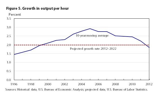
Healthy productivity growth will be important to the economy going forward if the nation is to continue to sustain economic growth despite a declining rate of labor force participation. Total factor productivity, the component of structural productivity growth not accounted for by increases in labor quality or the ratio of capital to labor, is expected to grow at a rate of 1.1 percent per year, about equal to its long-run average. Output per hour is anticipated to increase at a rate of 2.0 percent per year from 2012–2022. This growth rate is slightly faster than the 1.9 percent annual growth experienced the prior decade but is still well in line with historical trends. (See figure 5 and table 11.)
| Category | Levels | Annual rate of change | |||||
|---|---|---|---|---|---|---|---|
| 1992 | 2002 | 2012 | 2022 | 1992–2002 | 2002–2012 | 2012–2022 | |
Labor supply (in millions, unless noted): | |||||||
Total population | 256.9 | 287.9 | 315.0 | 339.2 | 1.1 | 0.9 | 0.7 |
Civilian noninstitutional population ages 16 and older | 192.8 | 217.6 | 243.3 | 265.3 | 1.2 | 1.1 | .9 |
Civilian labor force | 128.1 | 144.9 | 155.0 | 163.5 | 1.2 | .7 | .5 |
Civilian household employment | 118.5 | 136.5 | 142.5 | 154.8 | 1.4 | .4 | .8 |
Nonfarm payroll employment | 108.7 | 130.4 | 133.7 | 149.1 | 1.8 | .2 | 1.1 |
Unemployment rate (percent) | 7.5 | 5.8 | 8.1 | 5.4 | -2.6 | 3.4 | -4.0 |
Productivity: | |||||||
Private nonfarm business output per hour (billions of chained 2005 dollars) | 36.9 | 46.4 | 55.7 | 67.8 | 2.3 | 1.9 | 2.0 |
| Sources: Historical data, U.S. Bureau of Economic Analysis, U.S. Bureau of Census, U.S. Bureau of Labor Statistics; projected data, U.S. Bureau of Labor Statistics. | |||||||
When projecting over a 10-year horizon, economists must balance prior trends with expectations for the future. Some areas of the economy behave less regularly than other areas, making them more difficult to predict. Often, exogenous assumptions must be made (such as those presented earlier), some of which can significantly influence the outcome of the model.
For the 2022 projections, one source of uncertainty comes from the projected labor force. As women entered the workforce in the 1960s, the labor force participation rate rose steadily, peaking in the late 1990s. As the nation’s demographic shift took hold, participation rates declined as more individuals left the labor force for retirement, a trend that sped up rapidly during the recession. During a recession, a cyclical drop in participation rates is typical, since unemployed workers may be discouraged by the poor labor market conditions and may elect to stop their job search in favor of returning to school, staying at home to care for children or relatives, or engaging in other nonlabor activities. As labor markets improve, these individuals gradually return to work and the labor force participation rate improves. A great deal of debate exists regarding what portion of the recent declines in the participation rate could be attributed to cyclical dynamics and what portion are driven by the compositional effect of the aging of the baby-boom generation.26 BLS expects that demographics will precipitate a continued decline in the labor force participation rate. If this assumption is incorrect or if the recovery proves strong enough to lure retirees and discouraged workers back into the labor force, stronger than anticipated growth could result.
Instabilities in the global economy continually present a great deal of risk in the model. Beginning in 2009, a sovereign debt crisis emerged in several nations belonging to the Eurozone—namely Spain, Greece, Ireland, Portugal, and Cyprus—in which governments accrued massive levels of debt and were no longer able to borrow at reasonable rates or pay interest on their existing loans. Because of their shared currency, these nations’ options were limited and the risk of contagion to other nations was high. Eurozone nations were able to maintain the integrity of the currency by providing bailouts and financial support to some governments while the European Central Bank offered several long-term refinancing options to central banks.27 The Euro area recovery is nascent, and further debt crises could upset the balance that has been struck.28 Unemployment remains high in many nations, and the forecast for growth is weak. Though the situation has stabilized in recent months, it is still of concern to the projections since, as a unit, the EU is the largest trading partner of the United States. A declining situation in the EU would slow U.S. exports and hamper growth possibilities.
Fiscal policy uncertainty at home remains a substantial risk in the projections as well. When the 2022 projections were finalized for publication, the nation was only beginning to feel the effects of the sequester. Even with the reductions in spending resulting from the BCA, deficits are projected to rise again in the latter half of the coming decade on the basis of current legislation. Meaningful reform to entitlement programs, further cuts to discretionary spending, or increased revenues will be needed to keep deficits under control. The MA/US model assumes spending cuts that ultimately exceed those laid out in the BCA, but the likelihood and timing of further cuts are highly unpredictable. In recent years, Congress has relied on a series of temporary solutions to remedy issues with the federal budget, tax rates, and the debt ceiling. The additional uncertainty created by short-term solutions to these problems may have hampered businesses and consumer activity and could continue to do so in the future.
A final area of uncertainty in the projections is the assumption that future productivity growth will be strong. Productivity growth sank in the late 2000s. A spike followed the 2007–2009 recession, characteristic of economic downturns as firms attempt to maintain production levels while cutting back labor hours. In the years since, growth in output per hour has remained less than 1.0 percent per year. In a working paper for the National Bureau of Economic Research, Robert Gordon argues that the Web and computer revolution may have already realized its greatest benefits—nearly all businesses have a Web presence now, and many of the aspects of life that can be automated already have been.29 Rather than technology creating more efficient ways of working or replacing human labor with machines, the focus has shifted to making things smaller and more portable, which does not produce tremendous gains in productivity. It may take a new technological revolution to return to the growth rates seen in prior decades. Without meaningful growth in productivity, growth in output will be hindered.
To assess the degree to which varying areas of uncertainty pose risks to the projections, BLS performed a sensitivity analysis on several components. The impacts on the model results vary but are in line with what would be predicted by theory.
Projected labor force growth is forecasted at 0.5 percent per year over the next decade. To reach the expected unemployment rate of 5.4 percent in 2022, an increase in household employment of 102,500 people per month is needed. If the labor force were to grow 0.1 percent faster across the forecast period, an additional 12,500 employed people per month—1.5 million additional employed people over the decade—would be required to achieve the same unemployment rate. Faster labor force growth would also increase the GDP growth rate by 0.1 percentage point and would result in a personal savings rate of 2.7 percent, a full point lower than the baseline forecast.
A decrease in productivity would result in slower GDP growth and a lower unemployment rate. All else equal, a decrease of 0.1 percentage points in the growth of output per hour, attributable to slower growth in total factor productivity, lowers annual GDP growth to 2.5 percent from 2.6 percent in the baseline forecast. With lower productivity, more workers are needed to maintain output levels. Therefore, household employment growth rises to 12.7 million people over the decade, a difference of 0.5 million people from the baseline scenario, resulting in an unemployment rate of 5.1 percent. A lower unemployment rate drives the expected federal funds rate 0.6 percentage points higher, to 5.2 percent. The personal savings rate in 2022 increases 0.5 percentage points, resulting in a rate of 4.2 percent.
If the average federal personal tax rate is increased by 1.0 percent across the projections period, annual GDP growth falls by 0.1 percentage points as compared with the baseline. Growth in PCE also declines by 0.1 percentage point, to an annual rate of 2.5 percent. The unemployment rate in 2022 rises to 6.0 percent, 0.6 point higher than the baseline. The federal deficit is much smaller, at 2.7 percent of nominal GDP, compared with 3.6 percent of nominal GDP in the baseline projections. Interest-bearing debt held by the public declines accordingly to 71.7 percent of GDP, 4.6 percentage points lower than the baseline estimate of 76.3 percent.
STRUCTURAL CHANGES TO THE ECONOMY and the nation’s on-going demographic shift will be the driving forces in GDP growth over the next decade. In this set of projections, output growth will be somewhat slower than was estimated in prior publications. Resurgence in investment will be important to boosting productivity and counteracting the impacts of slow labor force growth and cuts in federal spending. Patterns of consumption will shift as the needs of an aging population dominate purchasing decisions. The recovery is expected to be gradual but persistent, bringing the unemployment down and returning the macroeconomy to a more stable position.
Maggie C. Woodward, "The U.S. economy to 2022: settling into a new normal," Monthly Labor Review, U.S. Bureau of Labor Statistics, December 2013, https://doi.org/10.21916/mlr.2013.43
1 Historical data come from the National Income and Product Accounts as of June 26, 2013, and are published by the Bureau of Economic Analysis. Data are available online at https://www.bea.gov/. Because the projections data are finalized well before publication, revised historical data, including changes made during the 2013 NIPA (National Income and Product Accounts) Comprehensive Revision, were not incorporated prior to publication. Unless noted, levels cited are measured in chain-weighted 2005 dollars. For a discussion of the uses and limitations of chain-type indexes, see J. Steven Landefeld and Robert P. Parker, “BEA’s chain indexes, time series, and measures of long-term economic growth,” Survey of Current Business, May 1997, https://apps.bea.gov/scb/account_articles/national/0597od/maintext.htm.
2 See Sylvain Leduc and Zheng Liu, “Uncertainty and the slow labor market recovery,” Economic Letter, no. 2013-21 (Federal Reserve Bank of San Francisco, July 22, 2013), http://www.frbsf.org/economic-research/publications/economic-letter/2013/july/us-labor-market-uncertainty-slow-recovery/.
3 The National Bureau of Economic Research is responsible for determining the official start and end dates of recessions in the United States. The most recent recession began in December 2007 and lasted through June 2009.
4 See speech by Ben S. Bernanke, “The economic recovery and economic policy,” given at the New York Economic Club, November 20, 2012.
5 See Brian Lucking and Daniel Wilson, “U.S. fiscal policy: Headwind or tailwind?” Economic Letter, no. 2012-20 (Federal Reserve Bank of San Francisco, July 2, 2012), http://www.frbsf.org/economic-research/publications/economic-letter/2012/july/us-fiscal-policy/.
6 For more information, see the Macroeconomic Advisers website, http://www.macroadvisers.com/.
7 In a full-employment economy, the unemployment rate is equal to the nonaccelerating inflation rate of unemployment (NAIRU). Labor supply and labor demand are in equilibrium; any existing unemployment is frictional.
8 For more information on BLS labor force projections, see accompanying article, “Labor force projections to 2022: the labor force participation rate continues to fall,” by Mitra Toossi, in this projections series of the Monthly Labor Review.
9 The Congressional Budget Office (CBO) prepares semiannual budget forecasts based on current laws. The most recent estimates available at the time of this writing were CBO “Updated budget projections: fiscal years 2013 to 2023,” May 14, 2013, http://cbo.gov/publication/44172.
10 See transcript of Chairman Bernanke’s Press Conference, June 19, 2013, http://www.federalreserve.gov/mediacenter/files/FOMCpresconf20130619.pdf.
11 For more information, see “Press Release” (Board of Governors of the Federal Reserve System, December 12, 2012), http://www.federalreserve.gov/newsevents/press/monetary/20121212a.htm.
12 Price projections for 2013–2022 are incorporated into the model. See Annual Energy Outlook 2013 (U.S. Energy Information Administration, April 15, 2013), http://www.eia.gov/forecasts/aeo/index.cfm.
13 See Dowell Myers and SungHo Ryu, “Aging baby boomers and the generational housing bubble: foresight and mitigation of an epic transition,” Journal of the American Planning Association, vol. 74, February 8, 2008, pp. 17–33, http://dx.doi.org/10.1080/01944360701802006.
14 See IHS Automotive: Polk, company news reported, “Polk finds average age of light vehicles continues to rise,” August 6, 2013, https://www.polk.com/company/news/polk_finds_average_age_of_light_vehicles_continues_to_rise.
15 See Kyle Fee and Daniel Hartley, “Housing recovery?” Economic Trends (Federal Reserve Bank of Cleveland, May 22, 2013).
16 See Andrew D. Paciorek, “The long and the short of household formation” (Finance and Economics Discussion Series, Federal Reserve Board, April 1, 2013), no. 2013-26, http://www.federalreserve.gov/pubs/feds/2013/201326/201326pap.pdf.
17 See Margaret Jacobson and Filippo Occhino, “The delayed recovery of investment in nonresidential structures,” Economic Trends (Federal Reserve Bank of Cleveland, May 6, 2013).
18 For more information, see “World economic outlook update: growing pains,” Annual Report (Washington, DC: International Monetary Fund, July 9, 2013), http://www.imf.org/external/pubs/ft/weo/2013/update/02/index.htm.
19 Receipts and expenditures for the federal government and for state and local governments are measured in current dollars.
20 Deficits are measured in current dollars. See “The budget and economic outlook: fiscal years 2013 to 2023” (Congressional Budget Office, February 5, 2013), http://cbo.gov/publication/43907.
21 See Brian Lucking and Daniel Wilson, “Fiscal headwinds: Is the other shoe about to drop?” Economic Letter, no. 2013-16 (Federal Reserve Board of San Francisco, June 3, 2013), http://www.frbsf.org/economic-research/publications/economic-letter/2013/june/fiscal-headwinds-federal-budget-policy/.
22 See Linda J. Bilmes, “The financial legacy of Iraq and Afghanistan: how wartime spending decisions will constrain future national security budgets,” Working Paper RWP13-006 (Harvard Kennedy School Faculty, Cambridge, Massachusetts, March 2013).
23 Personal income and its components are measured in current dollars.
24 See Daniel Aaronson and Scott Brave, “Estimating the trend in employment growth” Chicago Fed Letter, no. 312 (Federal Reserve Bank of Chicago, July 2013), http://www.chicagofed.org/digital_assets/publications/chicago_fed_letter/2013/cfljuly2013_312.pdf.
25 See A. Michael Spence, “The evolving structure of the American economy and the employment challenge,” Working Paper (Council on Foreign Relations, March 2011); Nir Jaimovich and Henry E. Siu, “The trend is the cycle: job polarization and jobless recoveries,” Working Paper 18334 (National Bureau of Economic Research, August 2012), http://www.nber.org/papers/w18334; and Robert B. Reich, “Manufacturing jobs are never coming back,” Forbes, May 2009, http://www.forbes.com/2009/05/28/robert-reich-manufacturing-business-economy.html.
26 For more information, see Leila Bengali, Mary Daly, and Rob Valletta, “Will labor force participation bounce back?” Economic Letter, no. 2013-14 (Federal Reserve Board of San Francisco, May 13, 2013), http://www.frbsf.org/economic-research/publications/economic-letter/2013/may/will-labor-force-participation-bounce-back/.
27 See The Economist Free exchange blog, “Draghi strikes back II,” February 29, 2012, http://www.economist.com/blogs/freeexchange/2012/02/europes-central-bank-and-euro-crisis.
28 See “Euro-zone economies: Mirabile dictu,” The Economist, August 15, 2013, http://www.economist.com/news/finance-and-economics/21583650-recovery-last-no-revelation-mirabile-dictu.
29 See Robert J. Gordon, “Is U.S. economic growth over? Faltering innovation confronts the six headwinds,” Working Paper 18315 (National Bureau of Economic Research, August 2012), http://www.nber.org/papers/w18315, and Erik Brynjolfsson and Andrew McAfee, “Jobs, productivity and the great decoupling,” New York Times, December 11, 2012, http://www.nytimes.com/2012/12/12/opinion/global/jobs-productivity-and-the-great-decoupling.html?_r=1&.