An official website of the United States government
An official website of the United States government
The .gov means it's official.
Federal government websites often end in .gov or .mil. Before sharing sensitive information,
make sure you're on a federal government site.
The site is secure.
The
https:// ensures that you are connecting to the official website and that any
information you provide is encrypted and transmitted securely.
14-2237-DAL
Wednesday, December 31, 2014
Employment rose in Oklahoma’s three large counties from June 2013 to June 2014, the U.S. Bureau of Labor Statistics reported today. (Large counties are defined as those with employment of 75,000 or more as measured by 2013 annual average employment.) Regional Commissioner Stanley W. Suchman noted that Cleveland County had the largest increase, up 2.1 percent, followed by Tulsa (1.6 percent) and Oklahoma (1.0 percent). (See table 1.)
Employment nationwide advanced 2.0 percent during the 12-month period as 305 of the 339 largest U.S. counties registered increases. Weld, Colo., recorded the fastest employment gain in the country, up 8.9 percent. Atlantic, N.J. experienced the largest over-the-year decrease among these counties with a loss of 1.6 percent.
Among the three largest counties in Oklahoma, employment was highest in Oklahoma County (442,400) in June 2014. Tulsa and Cleveland Counties had employment levels of 342,900 and 78,400, respectively. Together, the three largest Oklahoma counties accounted for 54.7 percent of total employment within the state. Nationwide, the 339 largest counties made up 71.8 percent of total U.S. employment.
All three large Oklahoma counties experienced average weekly wage gains from the second quarter of 2013 to the second quarter of 2014. Tulsa County recorded the fastest rate of increase in average weekly wages, up 3.6 percent. (See table 1.) Tulsa County also had the highest average weekly wage among the state’s largest counties at $894, closely followed by Oklahoma County ($891). Nationally, the average weekly wage increased 2.1 percent from a year ago to $940 in the second quarter of 2014.
Employment and wage levels (but not over-the-year changes) are also available for the 74 counties in Oklahoma with employment below 75,000. In all but one of these smaller counties, wage levels were below the national average. (See table 2.)
Large county wage changesTulsa County’s 3.6-percent rise in average weekly wages from the second quarter of 2013 to the second quarter of 2014 ranked 32nd among the nation’s 339 largest counties and was well above the U.S. average rate of increase (2.1 percent). Advancing at a slower pace, wages in Oklahoma and Cleveland recorded over-the-year increases of 1.9 percent and 1.8 percent, respectively. (See table 1.)
Nationally, 312 of the 339 largest counties registered over-the-year wage increases. Midland, Texas, experienced the largest wage gain in the nation, up 9.0 percent. Douglas, Colo., had the second largest overall increase (8.8 percent), followed by Hillsborough, N.H. and Collier, Fla. (7.4 and 6.8 percent, respectively).
Nationwide, 22 of the largest counties registered wage declines during the period. Williamson, Texas, experienced the largest decrease in average weekly wages with a loss of 2.7 percent over the year. Westchester, N.Y., had the second largest wage decline (-1.6 percent), followed by Lake, Ind. (-1.4 percent), and Bibb, Ga. (-1.3 percent).
Large county average weekly wagesWeekly wages in the state’s three large counties were below the national average of $940 per week. In the second quarter of 2014, average wages in Tulsa County ($894) ranked 148th and Oklahoma County ($891) ranked 151st, both in the middle of the national ranking of the 339 largest counties. In contrast, wages in Cleveland County ($716) ranked among the lowest, at 319th. (See table 1.)
Nationwide, average weekly wages were higher than the U.S. average ($940) in 109 of the 339 largest counties. Santa Clara, Calif., held the top position among the highest-paid large counties with an average weekly wage of $1,886. San Mateo, Calif., was second with an average weekly wage of $1,740, followed by New York, N.Y. ($1,732).
Two-thirds of the largest U.S. counties (230) reported average weekly wages below the national average in the second quarter of 2014. The lowest wage was reported in Horry, S.C. ($548), followed by the Texas counties of Cameron ($585) and Hidalgo ($608). Wages in these lowest-ranked counties were less than one-third of the average weekly wage reported for the highest-ranked county, Santa Clara, Calif. ($1,886).
Average weekly wages in Oklahoma's smaller countiesAmong the 74 smaller counties in Oklahoma – those with employment below 75,000 – Kingfisher ($979) was the sole county to report average weekly wages above the $940 national average. Including Kingfisher, three others – Woodward ($922), Beckham, and Washington (both at $898 per week) – were among the highest-paid smaller counties in the state. Cimarron County reported the lowest average weekly wage in the state with an average of $500 in the second quarter of 2014. (See table 2.)
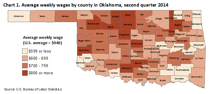
When all 77 counties in Oklahoma were considered, 14 reported average wages under $600 per week, 27 registered wages from $600 to $699, 23 had wages from $700 to $799, 13 had wages of $800 or more. (See chart 1.) The higher-paying counties were concentrated around the larger metropolitan areas of Oklahoma City and Tulsa, as well as smaller cities including Elk City, Enid, and Woodward. The lower-paying counties, those with weekly wages under $600, were generally located in the eastern third of the state.
Additional statistics and other informationQCEW data for states have been included in this release in table 3. For additional information about quarterly employment and wages data, please read the Technical Note or visit www.bls.gov/cew.
Employment and Wages Annual Averages Online features comprehensive information by detailed industry on establishments, employment, and wages for the nation and all states. The 2013 edition of this publication contains selected data produced by Business Employment Dynamics (BED) on job gains and losses, as well as selected data from the first quarter 2014 version of the news release. Tables and additional content from Employment and Wages Annual Averages 2013 are now available online at www.bls.gov/cew/publications/employment-and-wages-annual-averages/2013/home.htm.
Information in this release will be made available to sensory impaired individuals upon request. Voice phone: 202-691-5200; Federal Relay Service: 1-800-877-8339.
Average weekly wage data by county are compiled under the Quarterly Census of Employment and Wages (QCEW) program, also known as the ES-202 program. The data are derived from summaries of employment and total pay of workers covered by state and federal unemployment insurance (UI) legislation and provided by State Workforce Agencies (SWAs). The 9.4 million employer reports cover 137.8 million full- and part-time workers. The average weekly wage values are calculated by dividing quarterly total wages by the average of the three monthly employment levels of those covered by UI programs. The result is then divided by 13, the number of weeks in a quarter. It is to be noted, therefore, that over-the-year wage changes for geographic areas may reflect shifts in the composition of employment by industry, occupation, and such other factors as hours of work. Thus, wages may vary among counties, metropolitan areas, or states for reasons other than changes in the average wage level. Data for all states, Metropolitan Statistical Areas (MSAs), counties, and the nation are available on the BLS Web site at www.bls.gov/cew/; however, data in QCEW press releases have been revised (see Technical Note below) and may not match the data contained on the Bureau’s Web site.
QCEW data are not designed as a time series. QCEW data are simply the sums of individual establishment records reflecting the number of establishments that exist in a county or industry at a point in time. Establishments can move in or out of a county or industry for a number of reasons–some reflecting economic events, others reflecting administrative changes.
The preliminary QCEW data presented in this release may differ from data released by the individual states as well as from the data presented on the BLS Web site. These potential differences result from the states’ continuing receipt, review and editing of UI data over time. On the other hand, differences between data in this release and the data found on the BLS Web site are the result of adjustments made to improve over-the-year comparisons. Specifically, these adjustments account for administrative (noneconomic) changes such as a correction to a previously reported location or industry classification. Adjusting for these administrative changes allows users to more accurately assess changes of an economic nature (such as a firm moving from one county to another or changing its primary economic activity) over a 12-month period. Currently, adjusted data are available only from BLS press releases.
| Area | Employment | Average Weekly Wage (1) | |||||
|---|---|---|---|---|---|---|---|
| June 2014 (thousands) | Percent change, June 2013-14 (2) | National ranking by percent change (3) | Average weekly wage | National ranking by level (3) | Percent change, second quarter 2013-14 (2) | National ranking by percent change (3) | |
|
United States (4) |
137,776.40 | 2.0 | -- | $940 | -- | 2.1 | -- |
|
Oklahoma |
1,578.00 | 1.0 | -- | 816 | 33 | 2.6 | 12 |
|
Cleveland, Okla. |
78.4 | 2.1 | 129 | 716 | 319 | 1.8 | 167 |
|
Oklahoma, Okla. |
442.4 | 1.0 | 244 | 891 | 151 | 1.9 | 156 |
|
Tulsa, Okla. |
342.9 | 1.6 | 177 | 894 | 148 | 3.6 | 32 |
|
(1) Average weekly wages were calculated using unrounded data. |
|||||||
|
Note: Data are preliminary. Covered employment and wages includes workers covered by Unemployment Insurance (UI) and Unemployment Compensation for Federal Employees (UCFE) programs. |
|||||||
| Area | Employment June 2014 |
Average Weekly Wage (1) |
|---|---|---|
|
United States (2) |
137,776,364 | $940 |
|
Oklahoma |
1,577,969 | 816 |
|
Adair |
4,656 | 606 |
|
Alfalfa |
1,731 | 810 |
|
Atoka |
3,172 | 587 |
|
Beaver |
1,868 | 732 |
|
Beckham |
11,785 | 898 |
|
Blaine |
3,138 | 702 |
|
Bryan |
14,865 | 657 |
|
Caddo |
6,707 | 692 |
|
Canadian |
31,727 | 774 |
|
Carter |
23,815 | 775 |
|
Cherokee |
15,411 | 640 |
|
Choctaw |
4,151 | 567 |
|
Cimarron |
706 | 500 |
|
Cleveland |
78,381 | 716 |
|
Coal |
1,102 | 659 |
|
Comanche |
42,551 | 712 |
|
Cotton |
1,461 | 584 |
|
Craig |
5,490 | 635 |
|
Creek |
18,831 | 752 |
|
Custer |
13,361 | 759 |
|
Delaware |
8,893 | 566 |
|
Dewey |
1,499 | 774 |
|
Ellis |
1,312 | 797 |
|
Garfield |
26,995 | 857 |
|
Garvin |
9,716 | 850 |
|
Grady |
12,584 | 714 |
|
Grant |
1,438 | 874 |
|
Greer |
1,264 | 599 |
|
Harmon |
710 | 596 |
|
Harper |
1,239 | 657 |
|
Haskell |
3,383 | 550 |
|
Hughes |
3,132 | 602 |
|
Jackson |
9,361 | 660 |
|
Jefferson |
1,049 | 631 |
|
Johnston |
2,551 | 652 |
|
Kay |
18,588 | 730 |
|
Kingfisher |
6,027 | 979 |
|
Kiowa |
2,167 | 635 |
|
Latimer |
3,328 | 779 |
|
LeFlore |
13,429 | 670 |
|
Lincoln |
6,758 | 664 |
|
Logan |
7,246 | 639 |
|
Love |
4,861 | 628 |
|
Major |
2,941 | 808 |
|
Marshall |
4,588 | 639 |
|
Mayes |
12,209 | 769 |
|
McClain |
8,410 | 667 |
|
McCurtain |
10,965 | 614 |
|
McIntosh |
3,948 | 545 |
|
Murray |
5,983 | 656 |
|
Muskogee |
29,185 | 717 |
|
Noble |
4,578 | 759 |
|
Nowata |
1,687 | 570 |
|
Okfuskee |
2,406 | 589 |
|
Oklahoma |
442,412 | 891 |
|
Okmulgee |
9,626 | 635 |
|
Osage |
6,776 | 697 |
|
Ottawa |
11,643 | 581 |
|
Pawnee |
3,194 | 752 |
|
Payne |
33,483 | 767 |
|
Pittsburg |
16,007 | 773 |
|
Pontotoc |
17,099 | 707 |
|
Pottawatomie |
22,374 | 641 |
|
Pushmataha |
2,773 | 560 |
|
Roger Mills |
755 | 769 |
|
Rogers |
27,757 | 836 |
|
Seminole |
7,223 | 668 |
|
Sequoyah |
9,189 | 521 |
|
Stephens |
15,866 | 835 |
|
Texas |
9,869 | 689 |
|
Tillman |
1,952 | 627 |
|
Tulsa |
342,907 | 894 |
|
Wagoner |
9,173 | 675 |
|
Washington |
21,407 | 898 |
|
Washita |
2,179 | 710 |
|
Woods |
3,850 | 751 |
|
Woodward |
10,684 | 922 |
|
(1) Average weekly wages were calculated using unrounded data. |
||
|
Note: Covered employment and wages includes workers covered by Unemployment Insurance (UI) and Unemployment Compensation for Federal Employees (UCFE) programs. Data are preliminary. |
||
| State | Employment | Average weekly wage (1) | ||||
|---|---|---|---|---|---|---|
| June 2014 (thousands) | Percent change, June 2013-14 | Average weekly wage | National ranking by level | Percent change, second quarter 2013-14 | National ranking by percent change | |
|
United States (2) |
137776.4 | 2.0 | $940 | -- | 2.1 | -- |
|
Alabama |
1872.9 | 0.7 | 806 | 36 | 1.6 | 38 |
|
Alaska |
344.9 | 0.5 | 1,014 | 8 | 4.6 | 2 |
|
Arizona |
2486.0 | 1.9 | 888 | 21 | 1.3 | 43 |
|
Arkansas |
1168.1 | 1.5 | 745 | 47 | 1.5 | 41 |
|
California |
15905.6 | 2.8 | 1,072 | 6 | 2.4 | 15 |
|
Colorado |
2439.3 | 3.4 | 960 | 14 | 2.9 | 8 |
|
Connecticut |
1676.6 | 0.6 | 1,155 | 3 | 2.5 | 13 |
|
Delaware |
429.0 | 2.5 | 976 | 11 | 1.2 | 44 |
|
District of Columbia |
732.6 | 1.0 | 1,569 | 1 | -0.5 | 51 |
|
Florida |
7628.6 | 3.1 | 839 | 28 | 2.1 | 23 |
|
Georgia |
4036.3 | 3.1 | 882 | 22 | 1.7 | 35 |
|
Hawaii |
624.6 | 1.1 | 845 | 26 | 2.7 | 10 |
|
Idaho |
659.2 | 2.5 | 697 | 51 | 2.2 | 22 |
|
Illinois |
5836.9 | 1.5 | 988 | 10 | 1.9 | 32 |
|
Indiana |
2916.9 | 1.8 | 784 | 42 | 1.2 | 44 |
|
Iowa |
1547.8 | 1.6 | 780 | 43 | 3.0 | 7 |
|
Kansas |
1372.8 | 1.7 | 797 | 38 | 2.3 | 20 |
|
Kentucky |
1820.8 | 1.7 | 798 | 37 | 2.0 | 27 |
|
Louisiana |
1921.6 | 1.4 | 843 | 27 | 2.4 | 15 |
|
Maine |
610.4 | 0.8 | 746 | 46 | 2.1 | 23 |
|
Maryland |
2594.4 | 0.9 | 1,020 | 7 | 1.6 | 38 |
|
Massachusetts |
3407.0 | 1.4 | 1,158 | 2 | 2.4 | 15 |
|
Michigan |
4164.7 | 2.3 | 897 | 20 | 2.3 | 20 |
|
Minnesota |
2782.0 | 1.3 | 947 | 16 | 1.9 | 32 |
|
Mississippi |
1101.1 | 0.5 | 705 | 50 | 2.0 | 27 |
|
Missouri |
2703.2 | 1.3 | 818 | 31 | 1.9 | 32 |
|
Montana |
453.4 | 1.1 | 734 | 48 | 2.4 | 15 |
|
Nebraska |
956.2 | 1.4 | 756 | 45 | 2.7 | 10 |
|
Nevada |
1210.1 | 3.4 | 833 | 30 | 0.6 | 50 |
|
New Hampshire |
637.2 | 1.2 | 955 | 15 | 4.3 | 3 |
|
New Jersey |
3944.8 | 0.8 | 1,097 | 5 | 1.2 | 44 |
|
New Mexico |
801.0 | 0.6 | 794 | 40 | 1.7 | 35 |
|
New York |
8965.2 | 1.8 | 1,146 | 4 | 2.4 | 15 |
|
North Carolina |
4080.7 | 2.4 | 818 | 31 | 1.2 | 44 |
|
North Dakota |
453.0 | 4.4 | 936 | 17 | 5.5 | 1 |
|
Ohio |
5233.8 | 1.4 | 846 | 25 | 2.1 | 23 |
|
Oklahoma |
1578.0 | 1.0 | 816 | 33 | 2.6 | 12 |
|
Oregon |
1748.4 | 2.4 | 874 | 23 | 2.9 | 8 |
|
Pennsylvania |
5719.8 | 1.0 | 933 | 18 | 1.6 | 38 |
|
Rhode Island |
472.9 | 1.6 | 898 | 19 | 2.0 | 27 |
|
South Carolina |
1916.4 | 2.7 | 765 | 44 | 2.5 | 13 |
|
South Dakota |
422.9 | 1.4 | 712 | 49 | 3.3 | 4 |
|
Tennessee |
2755.7 | 1.8 | 836 | 29 | 2.0 | 27 |
|
Texas |
11402.8 | 3.0 | 973 | 13 | 3.1 | 5 |
|
Utah |
1297.5 | 2.9 | 796 | 39 | 1.7 | 35 |
|
Vermont |
307.0 | 1.0 | 813 | 35 | 0.7 | 49 |
|
Virginia |
3710.8 | 0.7 | 976 | 11 | 0.8 | 48 |
|
Washington |
3109.6 | 3.2 | 990 | 9 | 2.1 | 23 |
|
West Virginia |
711.3 | -0.3 | 792 | 41 | 1.4 | 42 |
|
Wisconsin |
2809.1 | 1.3 | 816 | 33 | 2.0 | 27 |
|
Wyoming |
295.3 | 1.6 | 871 | 24 | 3.1 | 5 |
|
Puerto Rico |
897.0 | -2.0 | 504 | (3) | 0.6 | (3) |
|
Virgin Islands |
37.8 | -2.2 | 728 | (3) | 2.8 | (3) |
|
(1) Average weekly wages were calculated using unrounded data. |
||||||
|
Note: Data are preliminary. Covered employment and wages includes workers covered by Unemployment Insurance (UI) and Unemployment Compensation for Federal Employees (UCFE) programs. |
||||||
Last Modified Date: Wednesday, December 31, 2014