Handbook of Methods > International Price Program

Handbook of Methods International Price Program Calculation

International Price Program: Calculation

The U.S. Import and Export Price Indexes are modified Laspeyres indexes that aggregate import and export price data. The prices used include directly collected establishment data, administrative trade data from the U.S. Census Bureau, and data from other alternative sources. Census Bureau data also form the basis for the sample frames for the establishment survey data and for the trade dollar value weights used in the Laspeyres calculation. (For more information on data sources and the sampling process, see the data sources and design sections.)

Aggregation

Prices are grouped into different classification systems that represent product or industry categories. Prices are then aggregated into price indexes using index formulas and trade dollar value shares, or weights. No matter the classification system, the calculation of prices into price indexes uses the same approach. As described before, only price indexes are published by the International Price Program.

For merchandise goods, the U.S. Import and Export Price Indexes are calculated using three different classification systems for aggregation of prices into price indexes. The classification systems are the U.S. harmonized tariff schedule for imports and schedule B statistical classification for exports (Harmonized System or HS), the North American Industry Classification System (NAICS), and the end-use classification system developed by the Bureau of Economic Analysis (BEA).

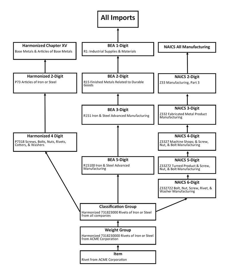
For the HS, NAICS, and BEA end-use classifications, the most detailed publishable price index levels are the four-digit, six-digit, and five-digit levels of aggregation, respectively. Larger digits signify a greater level of detail. The one-digit level is the top-level of aggregation for each classification system. For each classification group, aggregation to the all-goods import and export price indexes results in the same value for each measure regardless of the classification structure. Only one top-level goods import and one top-level goods export price index are published based on the end-use classification. For more information on how these classification systems relate to the U.S. Import and Export Price Indexes, see the concepts section.

The aggregation example in exhibit 3 shows how the price of an imported item (rivet), shown at the bottom of the exhibit, is mapped up through weight group and classification groups through the three classification systems to calculate different price indexes. A similar approach is used for exports.

The item prices at the classification group level that are aggregated to each stratum to calculate price indexes are composed of prices that are directly collected and from alternative data sources. For goods price indexes, the directly collected prices come from sampled data and from unit-value indexes calculated at the classification group level using administrative trade records. Together the directly collected prices and unit-value indexes form two non-overlapping subsets of item prices that cover the target population of merchandise goods trade. (For more information, see the data sources section.) The item prices used to calculate the transportation services price indexes are directly collected sampled data for air freight and a third-party data source for air passenger fares.

Services price indexes are aggregated to the product level only, given the incomplete coverage of services in import and export price indexes. For air transportation services, BLS calculates import and export air freight and air passenger price indexes using the balance of payments concept of payments and receipts between U.S. and foreign residents. In addition, inbound and outbound air freight price indexes are directional and measure the transportation of freight between the United States and foreign countries. At the lowest level of aggregation, items are mapped by locality using the U.S. Department of Transportation’s world area codes. At the most aggregated level, each air service measure is aggregated to an all-world price index for imports (exports) and inbound (outbound) separately. (For more information, see the concepts section.)

Note that price indexes are calculated for all strata and classifications, but not all calculated price indexes are published.

Exhibit 3. Aggregation example

flowchart of how import price indexes are aggregated

Index weights

The mapping structure and index weights are based upon a 2-year lagged classification structure and related fixed nominal dollar value of trade. Updates to classification structures and trade weights are made every year in January.

The weights used to calculate price indexes starting with the January release use the most recent final annual foreign trade measures published by the Census Bureau. Weights for aggregation from the classification group to the top-level price indexes are calculated for each 10-digit HS grouping and then aggregated to each detailed classification.

For sampled items, individual item weights are not available in the sample frame from which they are chosen. Instead, the weights are derived from the company weights based on trade weights within the 10-digit HS classification group from which the items are selected. For more detail on classification groups, see the design section. Company weights for sampled items within a classification group are based on dollar value and the probability of selection. The company weight is distributed evenly among the sampled items in the classification group. Items may represent multiple items in the same sample in an effort to reduce company burden. So, if similar items are sampled, only one may be collected where the item would retain the weight of each of the sampled items. In that case, the item weight within the sample would be multiplied by the number of items that the item represents. Items may also be sampled in multiple samples in which case the weights for each sample are summed. In effect, the item represents two or more items, one selected in each sample. For items derived from Census administrative trade values, the item and company weights are the same as the classification group weight because there is a one-to-one-to-one relationship between the item, weight group, and classification group.

The individual item price changes are aggregated into progressively more generalized groupings—defined as weight groups, classification groups, and strata—until an overall price change is calculated for all imports and all exports. Each weight group is a single company within a classification group, where the weight is derived by summing the company’s item weights. The weight groups are used to aggregate indexes to the classification group level. Classification groups are weighted by the 2-year lagged trade dollar values and are aggregated to the most detailed strata of each classification system to calculate price indexes for publication purposes.

Modified Laspeyres formula

BLS calculates all U.S. Import and Export Price Indexes using a Lowe, or modified fixed-quantity Laspeyres formula, with trade dollar values or their estimates as weights, which are updated annually on a 2-year lagged basis. Laspeyres indexes measure price change from a base period to the current period using the base period weights. In a Lowe price index, the weight reference period may precede the price reference period. The Laspeyres price index is a special case of the Lowe index where the weight reference period must match the price reference period. The second modification to the Laspeyres formula for calculating Import/Export Price Indexes is the use of a chained index instead of a fixed-base index. With chaining, the current-month price index is derived from the index value and price movement from the previous month rather than a base period. The index values from each month can then be chained back to the base period.

Below is the derivation of the modified fixed-quantity Laspeyres formula used to calculate all U.S. Import and Export Price Indexes.

$P_{t} = (\frac{\sum p_{i,t} q_{i,0}}{\sum p_{i, 0} q_{i, 0}}) (100) = (\frac{\sum \frac{p_{i,t}}{p_{i, 0}} p_{i,0} q_{i,0}}{\sum p_{i,0} q_{i,0}}) (100)$

$P_{t} = (\frac{\sum w_{i, 0} r_{i,t}}{\sum w_{i,0}}) (100) = (\frac{\sum w_{i,0} r_{i, t}}{\sum w_{i,0} r_{i,t - 1}}) (\frac{\sum w_{i,0} r_{i,t - 1}}{\sum w_{i,0}}) (100)$

$P_{t} = (\frac{\sum w_{i,0} r_{i,t}}{\sum w_{i,0} r_{i,t - 1}}) (P_{t - 1}) = ({STR}_{t})({LTR}_{t - 1})$

where

$P_{t}$ $P_{t}$ = index of collection items at time t,

$p_{i,t}$ = price of item i at time t,

$q_{i,0}$ = quantity of item i in base period 0,

$w_{i,0}$ = $(p_{i,0}) (q_{i,0})$ = total revenue of item i in base period 0,

$r_{i,t}$ = $(p_{i,t})/(p_{i,0})$ = long-term relative of item i at time t,

${STR}_{t}$ = $\frac{\sum w_{i,0} r_{i,t}}{\sum w_{i,0} r_{i,t - 1}}$ = short-term ratio of items at time t, and

${LTR}_{t}$ = = long-term relative of items at time t.

Estimating missing values

To maintain an uninterrupted time series, an estimated value is entered when there are missing data. Observations could be missing due to erratic reporting on the part of respondents, late data, insufficient administrative trade data, or strong seasonality in patterns of trade.

Exhibit 4 shows an example of how to address missing values. The ellipses represent a value which cannot be computed due to the missing value for item 2 in period 1. The items are used to derive the index values or long-term relatives (LTR) for the next level of aggregation, the company weight group. The missing price for item 2 in period 1 would adversely affect the index because neither the period 1 nor period 2 short-term relative (STR) can be derived for item 2.

Exhibit 4. Estimation example
Item	Element	Period 0	Period 1	Period 2
Item 1	Price	$10	$10	$10
	STR	1	1	1
	LTR	100	100	100
Item 2	Price	$20	^⁠1	$30
	STR	1	^⁠1	^⁠1
	LTR	100	^⁠1	150
Item 3	Price	$5	$10	$5
	STR	1	2	0.5
	LTR	100	200	100
Note: STR stands for short-term relative. LTR stands for long-term relative. ^⁠1 Data are not available. Source: U.S. Bureau of Labor Statistics.

In order to continue the series, values need to be estimated. The eventual method used for estimating missing values is linear interpolation once values are available before and after the missing period. When a period value is initially estimated before a subsequent value is available, cell mean imputation is used.

Cell mean imputation

For cell mean imputation, the STR from an item’s weight group would be used. However, if none of the items in the weight group have usable price data, then the STR would come from the classification group, the most detailed level HS stratum the classification group is mapped to, or potentially a more aggregated level in the HS classification structure. In the case of the lack of usable data for an item with an alternative data source, like Census administrative trade data, the item is unique to both the weight group and classification group, so the most detailed level HS stratum would be used to impute the item value. In all cases, imputation uses the HS structure from detailed to aggregated classification levels. The HS structure is a better match for price change than industry or end-use classification because HS is based on product type.

When one or more items are missing a price in a period a price can be cell mean imputed by multiplying the previous period’s price by the STR of the HS parent classification group. Prices are imputed so that when a usable price is received for a later period the index series can be continued by using the last imputed price as the denominator in computing an STR for the item. In cases where no price data are collected for a classification group, imputation will be the regular approach to establish a value for each period.

In the example below, assuming all three items are evenly weighted in this example, the other items in the weight group rise by 50 percent. The estimation of the missing value would be derived by taking the period 0 price of $20 and multiplying that by the average change for the weight group of 50 percent to get an imputed period 1 price of $30 as seen below in exhibit 5 (item 2, period 1).

Exhibit 5. Cell mean imputation example
Item	Element	Period 0	Period 1	Period 2
Item 1	Price	$10	$10	$10
	STR	1	1	1
	LTR	100	100	100
Item 2	Price	$20	$30	$30
	STR	1	1.5	1
	LTR	100	150	150
Item 3	Price	$5	$10	$5
	STR	1	2	0.5
	LTR	100	200	100
Note: STR stands for short-term relative. LTR stands for long-term relative. Source: U.S. Bureau of Labor Statistics.

The overall STR and LTR for the weight group can now be calculated for period 1.

${STR}_{1} = (\frac{\sum w_{i,0} r_{i, 1}}{\sum w_{i,0} r_{i, 0}}) = \frac{(1 * 100 + 1 * 150 + 1 * 200)}{(1 * 100 + 1 * 100 + 1 * 100)} = 1.5$

${LTR}_{1} = {STR}_{1} * {LTR}_{0} = 1.5 * 100.0 = 15 0$

Linear interpolation

Once a subsequent value is received, the estimation method switches from cell mean imputation to linear interpolation. The method uses the value for the item in periods before and after the period or periods where the price is not reported to linearly interpolate the middle value or values. Applying linear interpolation to the example in exhibit 4, the estimation of the missing value for the item in period 1 would be the midpoint of the item values in period 0 and period 2. That example is illustrated in exhibit 6.

Exhibit 6. Linear Interpolation example
Item	Element	Period 0	Period 1	Period 2
Item 1	Price	$10	$10	$10
	STR	1	1	1
	LTR	100	100	100
Item 2	Price	$20	$25	$30
	STR	1	1.25	1.2
	LTR	100	125	150
Item 3	Price	$5	$10	$5
	STR	1	2	0.5
	LTR	100	200	100
Note: STR stands for short-term relative. LTR stands for long-term relative. Source: U.S. Bureau of Labor Statistics.

Again, once the missing price for item 2 in period 1 is imputed, the STR and LTR for the weight group can be derived.

${STR}_{1} = (\frac{\sum w_{i,0} r_{i,1}}{\sum w_{i,0} r_{i,0}}) = \frac{(1 * 100 + 1 * 1 25 + 1 * 200)}{(1 * 100 + 1 * 100 + 1 * 100)} = 1. 42$

${LTR}_{1} = {STR}_{1} * {LTR}_{0} = 1. 42 * 100.0 = 1 42$

${STR}_{2} = (\frac{\sum w_{i,0} r_{i, 2}}{\sum w_{i,0} r_{i, 1}}) = \frac{(1 * 100 + 1 * 150 + 1 * 1 00)}{(1 * 100 + 1 * 1 25 + 1 * 2 00)} = 0.82$

${LTR}_{2} = {STR}_{2} * {LTR}_{1} = 0.82 * 1 42 .0 = 116.4$

With linear interpolation, in period 1, before the period 2 value is known, the item would initially be estimated using cell mean imputation and then would be revised using linear interpolation once the next actual value was reported. The linear interpolation method is preferred because it uses the value for the same item. However, because the next available value is not present in many cases, the fallback is to use the cell mean imputation methodology. The linear interpolation method is available because the import and export price indexes are revised in each of the three months after the indexes are first released. If no new value is received during the revision period, then the estimation is performed using cell mean imputation until a value is received.

Starting a series

The method for starting a price series in the Import and Export Price Indexes is known as initialization. This happens the month before the first price is received at initiation if that price is within the revision period when the item is initiated, and if not, the initialization happens the month before the first subsequent price is initiated. The technique is similar to the cell mean imputation technique used for missing prices. With initialization, the weight group LTR (if one is available) is used to start the series for an item. The regular cell mean imputation method is then used to fill in the missing STR.

Quality adjustment procedures and practices

Updates or modifications of a surveyed item sometimes affect the price or quality of the item. For example, a computer might be improved by adding more memory. The U.S. Import and Export Prices Indexes should reflect the pure price change in the index, not price changes because of changes in the quality of the item. For survey items, if the effect of the modification on price can be reliably estimated, a quality-adjusted price is used. If the value of the modification cannot be reliably estimated, the item is no longer considered to be the same item, and a new item is substituted into the survey.

Industry analysts evaluate the magnitude and impact of the modification to each item in the survey when the description is changed by the respondent. The respondent may be consulted in making this determination. If the modification does not change the class, general function, or purpose of the item and the respondent can quantify the change in the item description or modification, then a ratio of the previous and current price is set for that period. The intent is to adjust the new price in terms of the previous price, excluding the quality change. Thus, the item’s original price and subsequent prices will consistently reflect the original unmodified item, and the price change that is recorded for the item in each period will be solely the change in the market price. If the modification does change the item’s class, general function, or purpose, or the value of the change cannot be quantified, then the item is deemed to be a new product. Then, item substitution is done by an industry analyst, which is discussed below, in the section on substitution procedures and practices. For administrative trade and third-party items, quality adjusting is not possible. In general, administrative trade items are homogeneous and do not have as many updates and modifications as the items that are requested from respondents.

For computers, hedonic modeling is used to estimate the value of the quality change when this information is not available from the company. The term “hedonics” applies to any regression analysis that breaks out the price of a product into separate price-determining characteristics. Many products can be modeled as a bundle of product characteristics, and a quality change represents a change in the quality of one or more of the characteristics. The cost of the quality change is estimated by deriving implicit prices for each characteristic, whenever the quality of any of the characteristics is altered.

The hedonic models are ordinary least squares (OLS) regressions that estimate implicit prices for various price-determining characteristics. The regression uses many prices of many computers with many characteristics, and the independent variable regression coefficients are the estimated price change for a one-unit change in each price-determining characteristic. When a price change occurs for a computer and is due to a change in the characteristics of the model, the coefficient of the characteristic in the hedonic model is multiplied by the change in the characteristic to calculate the quality adjustment. This is the value of the quality adjustment, or VQA.

The general functional form of the hedonic model is shown in the equation below.

$P_{i} = β_{0} + \sum_{j = 1}^{n} β_{j} x_{ij} + ε_{i}$

where

$P_{i}$ = the price of good i,

$β_{0}$ = the constant term in the OLS regression,

$x_{ij}$ = characteristic j for good i,

$β_{j}$ = the coefficient on characteristic j, and

$ε_{i}$ = a random error term that is assumed to have a normal distribution with a mean of 0 and a standard deviation equal to $σ^{2}$ .

The constant term represents the base price. The coefficients are the implicit prices of the various characteristics. Price-determining characteristics may be modeled as continuous, discrete, or dummy variables.

Once the value of the quality adjustment is calculated, a link price is derived by taking the price of the new product in the current period and subtracting the value of the quality adjustment. Procedurally, the link price represents the value of the previous product in the current period (period 1). The period 1 STR is calculated as the percent change of the link price in period 1 to the price of the previous product in period 0. In period 2, the short-term relative is the change in the market price of the updated product from period 1 to period 2. Recall that only the price change is used in calculating price indexes. The different price levels between the previous product and the updated product are not used to calculate the price change. The advantage to this method is that the link price is being set in the period during which the quality adjustment takes place.

Substitution procedures and practices

For sampled items, item substitution is the replacement of a previously traded item with a new item from the same company and within the same commodity classification group. The previously priced item is discontinued because the item is no longer traded, or a change in item description is not quantifiable. In the month that the one-to-one replacement occurs, there is no short-term price ratio for either the discontinued or the new item. The new item will get a price ratio the next month once two prices are collected. The administrative trade items are derived from all trade in a specific classification, removing the need to account for item substitution.

Reweighting and rebasing

The U.S. Import and Export Price Indexes are reweighted annually due to changing patterns of trade. The weights used in the Laspeyres formula are the trade weights reported by the Census Bureau. These weights have a 2-year lag when annual trade data become available and applied to the indexes. For example, the weights for the indexes in 2025 are based on the import and export trade weights from the 2023 calendar year.

The best way to illustrate the need for annual reweighting is to give an example of the changing dollar values between weight years. In 2013, the petroleum area consisted of 12.6 percent of the total import trade dollar value in the import price indexes. By 2014, petroleum fell to 6.9 percent of the total import trade dollar value for the import price indexes, exhibiting a relatively sizable drop in value. If the indexes had not been reweighted on an annual basis, petroleum would have been overrepresented in the overall import price indexes.

To represent the least-biased weight of the Import and Export Price Indexes based on the trade value, the indexes need to be rebased to 100 for the weight year. The reason is that the relative weights or importance over time is based both on the fixed trade weights and the relative movement of the indexes as prices change. Indexes that fall at a relatively faster rate than other indexes have a smaller index value and will have less relative importance in the indexes; the reverse is true for indexes that rise at a faster rate relative to counterpart indexes.

Rebasing the published price indexes on an annual basis rather than holding the base period constant makes the indexes less user friendly for those who track the index value from month to month. Price indexes continuously published since 2000 have a fixed base period set equal to 2000 = 100. For indexes published subsequent to 2000, the index is based at 100 in the initial month of publication. In order to adjust the base year for usability, indexes are first rebased to the weight year. They are then calculated to update the price index values for the current month and three revision periods. Next, the indexes are subsequently rebased back to 2000 = 100 or to the first publication month = 100 for indexes published after 2000.

Seasonal adjustment

None of the import and export price indexes are seasonally adjusted. International trade happens worldwide with most items available regardless of the time of year. There is insufficient evidence for seasonality in import and export prices, although there is potentially seasonality in quantities which annual weights do not account for on a monthly basis. An effective method for eliminating seasonality is to look at the rolling 12-month percent changes rather than monthly percentage changes.

Variance estimates

Sampling variability results whenever a sample is used rather than the complete universe. Currently, standard errors are published on an annual basis for the all-import and all-export price indexes. (See Variance Estimates for Price Changes in the Import and Export Price Indexes). For each month in the previous calendar year, the standard error is available for the 1-month, 3-month, and 12-month percent changes. The standard error, the square root of the estimated variance, is a common measure used to derive confidence intervals for percent changes in the U.S. Import and Export Price Indexes. Confidence intervals can be used to determine if an index change is significantly different than zero.

For those price indexes that will be calculated with administrative trade data in place of directly collected survey data, no variance estimate will be calculated.

Sources of error

There are different types of errors that are introduced when calculating the U.S. Import and Export Price Indexes. One way to look at measurements of error is the difference between sampling error and nonsampling error. Sampling error is the error resulting from drawing a sample of imported and exported items to and from the United States, rather than using the entire universe of trade. Survey items have sampling error whereas the administrative trade items would not because they are derived from a census of all trade in a particular area. Sampling error is reduced with the use of administrative trade data that reflect the entire universe of trade.

Nonsampling error can take a number of different forms. One form is misspecification error, which takes place if the universe of data from which the sample is being drawn does not correctly measure the actual population. This type of error could result if trade is not reported or is misreported in import and export declarations used to construct the sample frame for the International Price survey. A second type of nonsampling error is nonresponse error. Each month, a subset of the items sampled do not have prices reported. This type of error results if the respondents and nonrespondents do not represent a similar cross section of the total universe. Another form of nonsampling error can be introduced from misreported prices.

One issue when deriving an estimate from a sample is the potential trade-off between variance and bias. Variance is a measure of how much the estimates derived from numerous samples differ from the true value of the estimate. Bias results when the expected value of the estimate is either higher or lower than the true value of what is being estimated. An estimate could have a high sampling variance and still be unbiased if the expected value of the estimate is equal to the true value. Likewise, an estimate may have small variation over numerous samples yet be biased if the expected value of the estimate deviates from the true value.

BLS strives to minimize both sampling and nonsampling error as much as possible. Sampling error is reduced by maintaining as many prices as possible to support an index, given resource and company burden constraints. Nonsampling error is reduced by subjecting the data to careful review and statistical analysis using automated checks and a staff of professional economists, as well as by employing methods to estimate missing observations.

With the administrative data source, there are a few potential sources of error. Processing error is one source of nonsampling error that is introduced with the use of the administrative trade data. Among the transaction records processed by the Census Bureau, some records have incomplete data and are not used in BLS calculations. Additionally, there is potential measurement error if the characteristics used to define a product variety inadequately explain the month-to-month price change movements. Furthermore, other records are analyzed and excluded from calculation because they are at the tails of the distribution of prices or quantities and are excluded in order to reduce the variability of unit prices and unit-value indexes. The exclusion of transactions with missing data and estimates at the tails of the distribution may result in bias or a skewed result if there is a repeatable pattern in either set of data, such that certain companies have more transactions with missing data or with widely variable prices. Nonsampling errors cannot be measured with current methods and there is little actual research on this topic for administrative data that represents the full population. Additional research to evaluate sources of error is underway. The research includes methods to adequately explain mean square error for index estimates that are constructed from the integration of administrative data and sampled survey data.

Replication and variance estimation

The reliability of sample data is evaluated by calculating the variance of index estimates using statistically selected subsamples of the sampled data. Specifically, to derive the standard error for survey items, a modified bootstrap method, applying rescaled sampling weights, is used to produce 150 replicate index set estimates from 150 simulated item set samples. Item set replicates are constructed according to the U.S. Import and Export Price Indexes 3-stage sample design. At both of the first two stages of sampling, it is possible for a selection to be either a certainty selection (i.e., the probability of selection is greater than the iteratively calculated sampling interval) or a probability selection. The replicate resampling method takes this into consideration by first partitioning the selected items within each sampling stratum m into those items that resulted from certainty establishment selections and those items resulting from probability establishment selections. The item set resulting from establishment certainty selections is further partitioned into two item sets: sampling classification group certainty selections and sampling classification group probability selections.

Thus, the set of all sampled items S is the union of these three partitions over all sampling stratum m

$S= ⋃_{m = 1}^{N} S_{m} = ⋃_{m = 1}^{N} (⋃_{p = 1}^{3} S_{m_{p}})$

where

N = the number of sampling strata, $p \in \{1,2,3\}$ ,

p = 1 for items selected from probability establishments,

p = 2 for items selected from probability sampling classification groups within certainty establishments, and

p = 3 for items selected from certainty sampling classification groups within certainty establishments.

Each bootstrap sampling, b, selects $n_{m_{p}}^{b}$ units within each partition of each sampling stratum as follows:

$n_{m_{p}}^{b} = \{\begin{matrix} n_{m_{p}} - 1 \\ 1 \end{matrix} \begin{matrix} n_{m_{p}} >1 \\ n_{m_{p}} = 1 \end{matrix}\}$

where

$n_{m_{p}}$ = the number of units originally sampled in partition p of sampling stratum m.

Bootstrap item weights are then calculated as

$w_{m_{p,j,i}}^{b} = \{\begin{matrix} w_{m_{p,j,i}} (\frac{n_{m_{p}}^{b} + 1}{n_{m_{p}}^{b}}) d_{m_{p,j}}^{b} \\ w_{m_{p,j,i}} \end{matrix} \begin{matrix} for n_{m_{p}} >1 \\ for n_{m_{p}} = 1 \end{matrix}\}$

where

$w_{m_{p,j,i}}^{b}$ = the bth replicate item weight for item i, within establishment j and sampling stratum partition $m_{p}$ $m_{p}$ ,

$w_{m_{p,j,i}}$ = the standard item weight for item i, within establishment j and sampling stratum partition , and

$d_{m_{p,j}}^{b}$ = the number of times establishment j within partition p of sampling stratum m, is selected in bootstrap sample b.

In the rare instances that $n_{m_{p}} = 1$ , a simple random sample of items within that establishment is selected. If only one item exists under this establishment singleton, that item is chosen with certainty.

For each of the 150 bootstrap samples, chained indexes of the desired length are calculated at all levels of aggregation using these modified item weights, original probabilities of selection, trade dollar values, and collected price data. For variance estimates, the variance is calculated across replicate percent change values for all published indexes as

$v_{B} = \frac{1}{150} \sum_{b = 1}^{150} {({\hat{θ}}_{b} - \hat{θ})}^{2}$

where

$\hat{θ}$ is the full sample estimate.

Last Modified Date: March 26, 2025