Employment rose in 7 of the 8 large counties in Indiana from March 2015 to March 2016, the U.S. Bureau of Labor Statistics reported today. (Large counties are defined as those with employment of 75,000 or more as measured by 2015 annual average employment.) Assistant Commissioner for Regional Operations Charlene Peiffer noted that Hamilton County had the largest increase, up 4.4 percent, followed by the counties of Elkhart (3.4 percent) and St. Joseph (3.0 percent). (See table 1.)

Nationally, employment advanced 2.0 percent from March 2015 to March 2016 as 318 of the 344 largest U.S. counties registered increases. Williamson, Tenn., had the largest percentage increase with a gain of 7.9 percent over the year. Midland, Texas, had the largest over-the-year percentage decrease in employment among the largest U.S. counties, with a loss of 9.0 percent.

Among the eight largest counties in Indiana, employment was highest in Marion County (583,600). Two other counties, Lake (183,300) and Allen (180,400), had employment levels above 150,000. Together, the eight largest Indiana counties accounted for 51.4 percent of total employment within the state. Nationwide, the 344 largest counties made up 72.6 percent of total U.S. employment.

Average weekly wages declined in 6 of the 8 large counties in Indiana from the first quarter of 2015 to the first quarter of 2016. Lake County had the largest percentage decrease in average weekly wages, down 4.2 percent. (See table 1.) Marion County recorded the highest average weekly wage among the state’s large counties at $1,069, followed by Hamilton County at $1,027. Nationally, the average weekly wage decreased 0.5 percent over the year to $1,043 in the first quarter of 2016.

Employment and wage levels (but not over-the-year changes) are also available for the 84 counties in Indiana with employment levels below 75,000. All but one of these smaller counties had average weekly wages below the national average. (See table 2.)

Large county wage changes

In addition to Lake County’s 4.2-percent decline in average weekly wages from the first quarter of 2015 to the first quarter of 2016, three other large counties in the state had wage declines greater than the national decrease of 0.5 percent: Vanderburgh (-3.0 percent), St. Joseph (-1.1 percent), and Allen (-0.7 percent). (See table 1.) Two of Indiana’s large counties registered wage increases over the year. Wages in Elkhart County increased 1.8 percent, ranking 47^th among the nation’s 344 large counties and wages in Tippecanoe County rose 0.2 percent and ranked 147^th nationwide.

Among the 344 largest U.S. counties, 167 had over-the-year decreases in average weekly wages in the first quarter of 2016. McLean, Ill., had the largest percentage decline in average weekly wages with a loss of 13.3 percent. Nationally, 164 large counties experienced over-the-year increases in average weekly wages. Clayton, Ga., had the largest percentage increase in average weekly wages with a gain of 15.5 percent.

Large county average weekly wages

As noted, Marion County ($1,069) had the highest average weekly wage in the state and ranked 79^th among the 344 largest U.S. counties. No other large county in Indiana had an average weekly wage that exceeded the national average of $1,043. Hamilton County ($1,027, 104^th) was the only other large county in Indiana to report an average weekly wage above $1,000. St. Joseph ($781) reported the lowest average weekly wage among the state’s large counties and ranked 299^th nationwide.

Nationally, weekly wages were higher than the U.S. average of $1,043 in 91 of the 344 largest counties. New York, N.Y., held the top position with an average weekly wage of $2,783. Santa Clara, Calif., was second at $2,210, followed by San Mateo, Calif. ($2,195); San Francisco, Calif. ($2,054); and Somerset, N.J. ($2,022). Among the 253 large counties with an average weekly wage below the U.S. average in the first quarter of 2016, Horry, S.C. ($587) reported the lowest wage.

Average weekly wages in Indiana’s smaller counties

Among the 84 counties in Indiana with employment below 75,000, only Martin County ($1,210) had an average weekly wage above the national average of $1,043. Average weekly wages in Brown ($480) and Ohio ($493) Counties were the lowest in the state. (See table 2.)

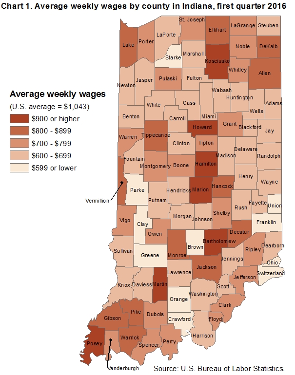
When all 92 counties in Indiana were considered, all but 2 had wages below the national average. Eleven reported average weekly wages less than $600, 39 had wages from $600 to $699, 22 reported wages from $700 to $799, 13 had wages from $800 to $899, and 7 had wages of $900 or more. (See chart 1.)

Additional statistics and other information

Quarterly data for states have been included in this release in table 3. For additional information about quarterly employment and wages data, please read the Technical Note or visit the QCEW Web site at www.bls.gov/cew/. Employment and Wages Annual Averages Online features comprehensive information by detailed industry on establishments, employment, and wages for the nation and all states. The 2015 edition of this publication contains selected data produced by Business Employment Dynamics (BED) on job gains and losses, as well as selected data from the fourth quarter 2015 version of the national news release. Tables and additional content from Employment and Wages Annual Averages 2015 are available online at www.bls.gov/cew/publications/employment-and-wages-annual-averages/2015/home.htm.

The County Employment and Wages release for second quarter 2016 is scheduled to be released on Wednesday, December 7, 2016.

Technical Note

Average weekly wage data by county are compiled under the Quarterly Census of Employment and Wages (QCEW) program, also known as the ES-202 program. The data are derived from summaries of employment and total pay of workers covered by state and federal unemployment insurance (UI) legislation and provided by State Workforce Agencies (SWAs). The 9.7 million employer reports cover 140.1 million full- and part-time workers. The average weekly wage values are calculated by dividing quarterly total wages by the average of the three monthly employment levels of those covered by UI programs. The result is then divided by 13, the number of weeks in a quarter. It is to be noted, therefore, that over-the-year wage changes for geographic areas may reflect shifts in the composition of employment by industry, occupation, and such other factors as hours of work. Thus, wages may vary among counties, metropolitan areas, or states for reasons other than changes in the average wage level. Data for all states, Metropolitan Statistical Areas (MSAs), counties, and the nation are available on the BLS Web site at www.bls.gov/cew/; however, data in QCEW press releases have been revised and may not match the data contained on the Bureau’s Web site.

QCEW data are not designed as a time series. QCEW data are simply the sums of individual establishment records reflecting the number of establishments that exist in a county or industry at a point in time. Establishments can move in or out of a county or industry for a number of reasons–some reflecting economic events, others reflecting administrative changes.

The preliminary QCEW data presented in this release may differ from data released by the individual states as well as from the data presented on the BLS Web site. These potential differences result from the states’ continuing receipt, review and editing of UI data over time. On the other hand, differences between data in this release and the data found on the BLS Web site are the result of adjustments made to improve over-the-year comparisons. Specifically, these adjustments account for administrative (noneconomic) changes such as a correction to a previously reported location or industry classification. Adjusting for these administrative changes allows users to more accurately assess changes of an economic nature (such as a firm moving from one county to another or changing its primary economic activity) over a 12-month period. Currently, adjusted data are available only from BLS press releases.

Information in this release will be made available to sensory impaired individuals upon request. Voice phone: (202) 691-5200; Federal Relay Service: (800) 877-8339.

Table 1. Covered employment and wages in the United States and the 8 largest counties in Indiana, first quarter 2016

Area	Employment			Average weekly wage (1)
	March 2016 (thousands)	Percent change, March 2015-16 (2)	National ranking by percent change (3)	Average weekly wage	National ranking by level (3)	Percent change, first quarter 2015-16 (2)	National ranking by percent change (3)
United States (4)	140,070.8	2.0	--	$1,043	--	-0.5	--
Indiana	2,949.5	1.9	--	853	33	-0.5	28
Allen, Ind.	180.4	1.9	176	835	252	-0.7	216
Elkhart, Ind.	126.3	3.4	55	849	234	1.8	47
Hamilton, Ind.	134.0	4.4	16	1,027	104	-0.4	201
Lake, Ind.	183.3	-0.4	321	850	232	-4.2	319
Marion, Ind.	583.6	1.4	235	1,069	79	-0.4	201
St. Joseph, Ind.	121.3	3.0	86	781	299	-1.1	224
Tippecanoe, Ind.	81.8	0.8	283	871	207	0.2	147
Vanderburgh, Ind.	105.6	0.8	283	799	285	-3.0	301
Footnotes: (1) Average weekly wages were calculated using unrounded data. (2) Percent changes were computed from quarterly employment and pay data adjusted for noneconomic county reclassifications. (3) Ranking does not include data for Puerto Rico or the Virgin Islands. (4) Totals for the United States do not include data for Puerto Rico or the Virgin Islands.
Note: Data are preliminary. Covered employment and wages includes workers covered by Unemployment Insurance (UI) and Unemployment Compensation for Federal Employees (UCFE) programs.

Table 3. Covered employment and wages by state, first quarter 2016

State	Employment		Average weekly wage (1)
	March 2016 (thousands)	Percent change, March 2015-16	Average weekly wage	National ranking by level	Percent change, first quarter 2015-16	National ranking by percent change
United States (2)	140,070.8	2.0	1043	--	-0.5	--
Alabama	1,902.6	1.6	842	37	-0.2	22
Alaska	317.6	-1.4	1028	15	-2	43
Arizona	2,679.8	2.8	918	23	-0.8	30
Arkansas	1,191.1	2.1	793	45	0.5	13
California	16,455.5	2.6	1206	6	0	20
Colorado	2,514.6	2.4	1057	13	-1.3	36
Connecticut	1,650.6	0.6	1362	3	-1.4	38
Delaware	429.7	1.5	1072	10	-3	48
District of Columbia	749.6	2.0	1766	1	0.4	14
Florida	8,301.8	3.5	887	27	0.2	18
Georgia	4,215.1	3.0	1008	17	1.9	2
Hawaii	645.1	1.4	896	26	1.7	3
Idaho	670.4	3.5	725	50	-1.5	39
Illinois	5,800.6	1.2	1126	7	-0.5	28
Indiana	2,949.5	1.9	853	33	-0.5	28
Iowa	1,518.2	0.9	844	36	-0.4	27
Kansas	1,362.3	0.4	833	38	-2	43
Kentucky	1,843.9	1.9	823	41	0.1	19
Louisiana	1,910.5	-0.8	860	32	-2.6	47
Maine	580.5	1.8	804	44	1.1	8
Maryland	2,591.7	1.9	1103	9	-0.8	30
Massachusetts	3,414.8	2.1	1327	4	-1	33
Michigan	4,163.7	2.1	976	20	0.7	11
Minnesota	2,750.1	1.5	1065	12	-1.2	34
Mississippi	1,121.0	1.7	713	51	0.4	14
Missouri	2,729.5	1.9	879	29	-0.3	25
Montana	447.8	1.8	751	49	0.3	16
Nebraska	956.6	1.4	817	42	0	20
Nevada	1,264.1	3.0	875	30	1.2	5
New Hampshire	635.1	1.9	998	18	1.6	4
New Jersey	3,909.7	2.4	1268	5	-1.7	41
New Mexico	800.4	0.0	792	46	-1.6	40
New York	9,042.2	2.0	1456	2	-0.3	25
North Carolina	4,220.3	3.0	928	22	-0.2	22
North Dakota	409.4	-6.2	908	25	-7.6	51
Ohio	5,236.2	1.8	913	24	-0.8	30
Oklahoma	1,578.6	-0.9	833	38	-4.1	49
Oregon	1,808.2	3.2	929	21	1.2	5
Pennsylvania	5,662.2	1.1	1012	16	-1.9	42
Rhode Island	464.6	1.9	985	19	-2.2	46
South Carolina	1,974.6	2.7	806	43	0.8	10
South Dakota	410.5	0.9	771	48	1.2	5
Tennessee	2,859.2	3.3	887	27	0.3	16
Texas	11,638.7	0.7	1066	11	-2.1	45
Utah	1,369.2	3.8	849	35	0.6	12
Vermont	304.6	0.1	832	40	1	9
Virginia	3,748.1	2.6	1057	13	-1.2	34
Washington	3,147.7	3.1	1121	8	3	1
West Virginia	683.9	-1.2	782	47	-1.3	36
Wisconsin	2,771.4	1.3	875	30	-0.2	22
Wyoming	267.9	-3.7	850	34	-4.7	50
Puerto Rico	895.2	-1.2	520	(3)	-0.4	(3)
Virgin Islands	38.6	0.4	769	(3)	2.9	(3)
Footnotes: (1) Average weekly wages were calculated using unrounded data. (2) Totals for the United States do not include data for Puerto Rico or the Virgin Islands. (3) Data not included in the national ranking.
Note: Data are preliminary. Covered employment and wages includes workers covered by Unemployment Insurance (UI) and Unemployment Compensation for Federal Employees (UCFE) programs.