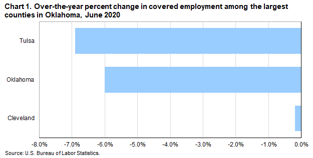
Employment fell in the three largest counties in Oklahoma from June 2019 to June 2020, the U.S. Bureau of Labor Statistics reported today. (Large counties are those with annual average employment levels of 75,000 or more in 2019.) Regional Commissioner Michael Hirniak noted that Tulsa County had the largest over-the-year decrease (-6.9 percent). (See chart 1 and table 1.)

National employment decreased 9.4 percent over the year, with all of the 357 largest U.S. counties reporting declines. Atlantic, NJ, had the largest over-the-year decrease in employment with a loss of 34.2 percent. Cleveland, OK, and Utah, UT, had the smallest over-the-year percentage decreases in employment, each with a loss of 0.2 percent.

Among the three largest counties in Oklahoma, employment was highest in Oklahoma County (438,200) in June 2020. The counties of Tulsa and Cleveland had employment levels of 338,100 and 80,900, respectively. Together, the three largest Oklahoma counties accounted for 56.3 percent of total employment within the state. Nationwide, the 357 largest counties made up 72.9 percent of total U.S. employment.

Employment and wage levels (but not over-the-year changes) are also available for the 74 counties in Oklahoma with employment below 75,000. Wage levels in all of these smaller counties were below the national average in the second quarter 2020. (See table 2.)

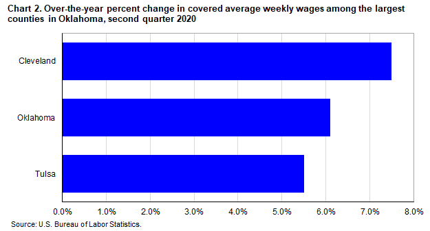
Large county wage changes

All three large Oklahoma counties reported average weekly wage gains from the second quarter of 2019 to the second quarter of 2020. (See chart 2.) However, the rates of wage gain in all large Oklahoma counties were below the national rate of 8.6 percent. Cleveland County had the largest gain (+7.5 percent).

Among the 357 largest counties in the United States, 352 had over-the-year wage increases. The increases in average weekly wages largely reflect substantial employment loss among lower-paid industries. Atlantic, NJ, had the largest percentage wage increase (+22.5 percent). Five large counties had wage declines during the period. Ector, TX, had the largest over-the-year percentage decrease (-6.6 percent).

Large county average weekly wages

Weekly wages in the state’s three large counties were all below the national average of $1,188 in the second quarter of 2020. Average weekly wages in Oklahoma County ($1,059) and Tulsa County ($1,017) ranked 190^th and 216^th, respectively, in the middle third of the large county national rankings. The average weekly wage in Cleveland County ($865) ranked 338^th, near the bottom of the 357 largest U.S. counties.

Among the largest U.S. counties, 101 reported average weekly wages above the U.S. average in the second quarter of 2020. Santa Clara, CA, had the highest average weekly wage at $3,045. Average weekly wages were at or below the national average in 256 counties. At $698 a week, Cameron, TX, had the lowest average weekly wage.

Average weekly wages in Oklahoma's smaller counties

All 74 smaller counties in Oklahoma – those with employment below 75,000 – reported average weekly wages below the national average of $1,188. Among these smaller counties, Washington posted the highest weekly wage, $1,007, followed by Grant ($949), Woodward ($943) and Kingfisher ($934). Cotton County reported the lowest average wage in the state at $556 per week, followed by McIntosh County at $611 per week. (See table 2.)

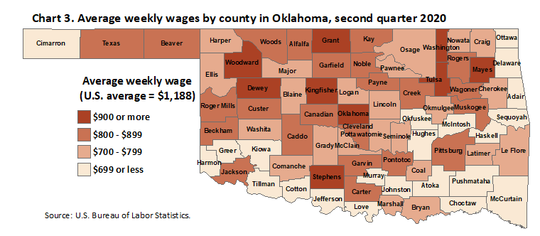
When all 77 counties in Oklahoma were considered, 16 reported average weekly wages of less than $700, 25 registered wages from $700 to $799, 25 had wages from $800 to $899, and 11 had average weekly wages of $900 or more. (See chart 3.) The higher-paying counties were located in and around the Oklahoma City and Tulsa metropolitan areas, as well as the smaller areas of Duncan and Woodward. The lower-paying counties, those with weekly wages under $700, were concentrated in the southern and eastern portions of the state.

Additional statistics and other information

QCEW data for states have been included in this release in table 3. For additional information about quarterly employment and wages data, please read the Technical Note or visit www.bls.gov/cew.

Employment and Wages Annual Averages Online features comprehensive information by detailed industry on establishments, employment, and wages for the nation and all states. The 2019 edition of this publication was published in September 2020. Tables and additional content from the 2019 edition of Employment and Wages Annual Averages Online are available at www.bls.gov/cew/publications/employment-and-wages-annual-averages/2019/home.htm. The 2020 edition of Employment and Wages Annual Averages Online will be available in September 2021.

Technical Note

Average weekly wage data by county are compiled under the Quarterly Census of Employment and Wages (QCEW) program, also known as the ES-202 program. The data are derived from summaries of employment and total pay of workers covered by state and federal unemployment insurance (UI) legislation and provided by State Workforce Agencies (SWAs). The average weekly wage values are calculated by dividing quarterly total wages by the average of the three monthly employment levels of those covered by UI programs. The result is then divided by 13, the number of weeks in a quarter. It is to be noted, therefore, that over-the-year wage changes for geographic areas may reflect shifts in the composition of employment by industry, occupation, and such other factors as hours of work. Thus, wages may vary among counties, metropolitan areas, or states for reasons other than changes in the average wage level. Data for all states, Metropolitan Statistical Areas (MSAs), counties, and the nation are available on the BLS web site at www.bls.gov/cew. However, data in QCEW press releases have been revised and may not match the data contained on the Bureau’s web site.

QCEW data are not designed as a time series. QCEW data are simply the sums of individual establishment records reflecting the number of establishments that exist in a county or industry at a point in time. Establishments can move in or out of a county or industry for a number of reasons–some reflecting economic events, others reflecting administrative changes.

The preliminary QCEW data presented in this release may differ from data released by the individual states as well as from the data presented on the BLS web site. These potential differences result from the states’ continuing receipt, review and editing of UI data over time. On the other hand, differences between data in this release and the data found on the BLS web site are the result of adjustments made to improve over-the-year comparisons. Specifically, these adjustments account for administrative (noneconomic) changes such as a correction to a previously reported location or industry classification. Adjusting for these administrative changes allows users to more accurately assess changes of an economic nature (such as a firm moving from one county to another or changing its primary economic activity) over a 12-month period. Currently, adjusted data are available only from BLS press releases.

Information in this release will be made available to individuals with sensory impairments upon request. Voice phone: (202) 691-5200; Federal Relay Service: (800) 877-8339.

Table 1. Covered employment and wages in the United States and the three largest counties in Oklahoma, second quarter 2020

Area	Establishments, second quarter 2020 (thousands)	Employment			Average weekly wage (1)
		June 2020 (thousands)	Percent change, June 2019–20 (2)	National ranking by percent change (3)	Second quarter 2020	National ranking by level (3)	Percent change, second quarter 2019–20(2)	National ranking by percent change (3)
United States (4)	10,451.0	135,114.4	-9.4	--	$1,188	--	8.6	--
Oklahoma	112.1	1,521.3	-6.3	--	940	44	4.4	49
Cleveland	6.1	80.9	-0.2	1	865	338	7.5	219
Oklahoma	28.6	438.2	-6.0	64	1,059	190	6.1	279
Tulsa	22.8	338.1	-6.9	95	1,017	216	5.5	302
(1) Average weekly wages were calculated using unrounded data. (2) Percent changes were computed from quarterly employment and pay data adjusted for noneconomic county reclassifications. (3) Ranking does not include data for Puerto Rico or the Virgin Islands. (4) Totals for the United States do not include data for Puerto Rico or the Virgin Islands.
Note: Data are preliminary. Covered employment and wages includes workers covered by Unemployment Insurance (UI) and Unemployment Compensation for Federal Employees (UCFE) programs.

Table 2. Covered employment and wages in the United States and all counties in Oklahoma, second quarter 2020

Area	Employment June 2020	Average weekly wage(1)
United States(2)	135,114,354	$1,188
Oklahoma	1,521,349	940
Adair	4,228	693
Alfalfa	1,294	879
Atoka	3,208	650
Beaver	1,253	821
Beckham	8,232	886
Blaine	2,821	803
Bryan	19,021	810
Caddo	7,118	856
Canadian	31,505	874
Carter	21,422	841
Cherokee	15,599	733
Choctaw	3,987	682
Cimarron	751	678
Cleveland	80,859	865
Coal	1,061	748
Comanche	39,239	779
Cotton	1,520	556
Craig	5,013	734
Creek	18,453	890
Custer	12,018	831
Delaware	9,201	687
Dewey	1,571	932
Ellis	1,149	775
Garfield	23,311	842
Garvin	9,354	910
Grady	11,509	790
Grant	1,360	949
Greer	901	681
Harmon	647	706
Harper	1,033	746
Haskell	3,038	622
Hughes	2,758	670
Jackson	9,345	885
Jefferson	1,063	690
Johnston	2,629	717
Kay	16,879	827
Kingfisher	6,529	934
Kiowa	1,820	715
Latimer	2,245	753
LeFlore	11,305	781
Lincoln	6,545	812
Logan	7,423	733
Love	6,255	658
Major	2,117	751
Marshall	4,159	795
Mayes	12,373	923
McClain	9,333	769
McCurtain	11,116	721
McIntosh	4,104	611
Murray	5,312	700
Muskogee	28,233	861
Noble	4,404	899
Nowata	1,809	793
Okfuskee	2,190	684
Oklahoma	438,161	1,059
Okmulgee	9,032	807
Osage	6,251	769
Ottawa	11,848	654
Pawnee	3,224	788
Payne	31,232	864
Pittsburg	14,350	869
Pontotoc	18,004	835
Pottawatomie	20,896	770
Pushmataha	2,276	695
Roger Mills	826	833
Rogers	25,568	900
Seminole	6,673	770
Sequoyah	9,426	652
Stephens	13,255	921
Texas	9,445	843
Tillman	1,541	711
Tulsa	338,097	1,017
Wagoner	9,369	884
Washington	17,959	1,007
Washita	1,833	799
Woods	3,112	839
Woodward	8,133	943
(1) Average weekly wages were calculated using unrounded data. (2) Totals for the United States do not include data for Puerto Rico or the Virgin Islands.
Note: Data are preliminary. Covered employment and wages includes workers covered by Unemployment Insurance (UI) and Unemployment Compensation for Federal Employees (UCFE) programs.

Table 3. Covered employment and wages by state, second quarter 2020

State	Establishments, second quarter 2020 (thousands)	Employment		Average weekly wage (1)
		June 2020 (thousands)	Percent change, June 2019–20	Second quarter 2020	National ranking by level	Percent change, second quarter 2019–20	National ranking by percent change
United States (2)	10,451.0	135,114.4	-9.4	$1,188	--	8.6	--
Alabama	131.2	1,868.7	-6.4	964	40	5.9	42
Alaska	22.7	296.2	-12.7	1,195	14	11.2	11
Arizona	170.7	2,708.4	-5.1	1,090	22	7.9	30
Arkansas	93.0	1,156.5	-5.5	924	47	7.3	33
California	1,633.1	15,911.2	-10.2	1,468	4	10.9	12
Colorado	216.4	2,545.9	-8.0	1,226	9	8.7	25
Connecticut	123.4	1,483.6	-12.3	1,407	6	11.3	9
Delaware	34.5	416.0	-9.3	1,156	17	9.0	22
District of Columbia	41.7	701.8	-10.0	1,987	1	11.7	7
Florida	738.0	8,113.8	-7.1	1,032	28	6.6	40
Georgia	307.2	4,196.0	-7.0	1,075	23	5.7	44
Hawaii	45.9	524.9	-20.1	1,108	21	12.0	6
Idaho	67.9	748.3	-2.3	882	50	7.6	32
Illinois	379.6	5,391.8	-11.3	1,218	10	8.6	26
Indiana	171.6	2,865.7	-7.3	960	41	5.6	45
Iowa	104.7	1,458.8	-8.0	978	36	8.4	27
Kansas	90.0	1,306.0	-7.0	969	38	7.1	34
Kentucky	125.4	1,754.0	-8.2	970	37	6.4	41
Louisiana	137.8	1,710.1	-11.0	985	34	6.7	39
Maine	53.8	572.5	-10.8	980	35	12.3	5
Maryland	175.8	2,430.3	-11.2	1,305	8	10.7	13
Massachusetts	263.1	3,178.8	-14.3	1,570	2	14.0	1
Michigan	268.5	3,850.9	-12.9	1,114	20	9.5	16
Minnesota	185.4	2,644.6	-10.5	1,200	13	9.0	22
Mississippi	73.8	1,063.1	-6.4	812	51	5.9	42
Missouri	215.9	2,622.2	-7.5	1,015	32	7.1	34
Montana	51.5	459.5	-4.9	919	48	9.1	19
Nebraska	72.9	932.3	-6.0	960	41	8.0	28
Nevada	85.9	1,191.6	-15.4	1,048	26	9.1	19
New Hampshire	54.8	605.4	-10.5	1,215	12	11.5	8
New Jersey	284.1	3,570.3	-14.6	1,376	7	11.3	9
New Mexico	62.4	757.0	-9.4	958	43	7.8	31
New York	652.0	8,142.6	-15.9	1,520	3	12.8	4
North Carolina	296.2	4,205.4	-6.9	1,038	27	6.9	37
North Dakota	32.4	390.1	-9.7	1,061	24	3.3	51
Ohio	302.3	5,049.8	-8.0	1,031	29	7.0	36
Oklahoma	112.1	1,521.3	-6.3	940	44	4.4	49
Oregon	160.9	1,789.3	-9.6	1,143	19	10.3	15
Pennsylvania	362.8	5,314.5	-11.1	1,170	16	9.2	18
Rhode Island	39.5	429.3	-13.2	1,172	15	13.1	3
South Carolina	144.4	1,991.0	-7.2	928	46	6.9	37
South Dakota	34.7	415.9	-5.9	912	49	9.0	22
Tennessee	171.1	2,847.2	-6.6	1,016	31	5.3	46
Texas	727.4	11,807.1	-6.3	1,156	17	5.0	47
Utah	111.6	1,474.8	-3.0	1,017	30	9.1	19
Vermont	26.1	271.8	-13.6	1,055	25	13.6	2
Virginia	283.3	3,635.2	-8.8	1,218	10	9.4	17
Washington	253.8	3,207.1	-8.4	1,424	5	10.6	14
West Virginia	51.3	634.9	-9.4	933	45	4.9	48
Wisconsin	179.2	2,690.0	-8.7	1,014	33	8.0	28
Wyoming	27.2	260.5	-9.6	965	39	3.7	50
Puerto Rico	46.1	798.7	-7.9	556	(3)	4.7	(3)
Virgin Islands	3.4	35.4	-7.0	1,016	(3)	6.9	(3)
(1) Average weekly wages were calculated using unrounded data. (2) Totals for the United States do not include data for Puerto Rico or the Virgin Islands. (3) Data not included in the national ranking.
Note: Data are preliminary. Covered employment and wages includes workers covered by Unemployment Insurance (UI) and Unemployment Compensation for Federal Employees (UCFE) programs.