Bureau of Labor Statistics > Job Openings and Labor Turnover Survey > Home

JOLTS State Estimates Methodology

Top

Synthetic Model
Composite Synthetic Model
Seasonal adjustment
Sample allocation
Reliability of estimates

The JOLTS sample of 21,000 establishments does not directly support the production of sample based state estimates. However, state estimates have been produced by combining the available sample with model-based estimates. JOLTS state-level estimates beginning in July 2026 will be released on an annual basis. BLS welcomes comments on the methodology used to produce these estimates.

These estimates consist of two major estimating models; the Synthetic model (an unpublished intermediate model) and the Composite Synthetic model (published historical series through the most current benchmark year). The Composite Synthetic model uses JOLTS microdata and Synthetic model estimates derived from monthly employment changes in microdata from the Quarterly Census of Employment and Wages (QCEW), and JOLTS published regional data.

The following outlines each model in a non-technical summary format. Each model is summarized separately, and answers the following:

What is the approach attempting to do?
What data inputs are used in the approach?
How does the approach attempt to use that data?
What data outputs are produced by the approach?
What limitations does the approach have?
What more needs to be done?

Synthetic Model

What approach?

The Synthetic approach uses data from the QCEW that have been linked longitudinally (Longitudinal Database—LDB), the QCEW-LDB. The Synthetic model attempts to convert QCEW-LDB monthly employment change microdata into JOLTS job openings, hires, quits, layoffs and discharges, and total separations data.

What data inputs?

All monthly employment changes for each record on the QCEW-LDB
JOLTS published regional estimates (regional JO, H, Q, LD, and TS)

How are data used?

Every record on the QCEW-LDB is classified as expanding, contracting, or stable based on monthly employment change.

For expanding records, the amount of employment growth is converted to JOLTS hires. They are given no separations.
For contracting records, the amount of employment decline is converted to JOLTS separations. They are given no hires.
For stable records, no attribution of JOLTS hires or separations is made.

The entire QCEW-LDB is summarized to the US Census regional level.
The QCEW-LDB regional summary is ratio adjusted to the JOLTS published regional estimate for hires and total separations.

For each region, the ratio of QCEW-LDB based regional hires and total separations to JOLTS published hires and total separations is calculated (Ratio-H for hires and Ratio-TS for total separations).
Each record on the QCEW-LDB within each US Census region will have their converted JOLTS data multiplied by Ratio-H and Ratio-TS, by region.
1. For expanding records, the amount of employment growth is then: (JOLTS hires×Ratio-H). They remain with no separations.
2. For contracting records, the amount of employment decline is then: (JOLTS separations×Ratio-TS). They remain with no hires.
3. For stable records, they remain with no JOLTS hires or separations.

To produce state-level estimates, sum the regional hires×Ratio-H by state to produce a state-level JOLTS hires estimate and sum the TS×Ratio-TS by state to produce a state-level JOLTS total separations estimate.

How are the outputs produced?

State-level JOLTS estimates for hires and total separations come directly from the model outlined above.
- Synthetic job openings are a function of the ratio of industry-regional job openings and hires. This ratio of published job openings to hires is applied to model hires estimates to derive model job opening estimates. Ratio-adjusting the JOLTS model hires and separations to the regional published JOLTS hires and separations estimates ensures that the JOLTS published churn rate is fully accounted for.
- Synthetic quits and layoffs and discharges are a function of the relative percentage of the individual components of total separations at the industry-regional level. The relative percentages of each component are applied to the model separations estimates to derive model quits and layoffs and discharges.

What are the limitations?

This approach is NOT meant to model individual QCEW-LDB data records. It would not be prudent to use this approach to model small populations (30 or fewer establishments). The model works best at the state-level, and while it is possible to model smaller populations, there potentially is a reduction in the strength of the model proportionate to the reduction in the size of the population being modeled
The model does generate state-level job openings and separations breakouts. However, these estimates are based upon ratios that are common across the region to which a state belongs. If there are significant differences in the ratio of job openings to hires or separations breakouts for any particular state (or set of states) within a region, the model cannot detect that and estimates will not reflect those differences.
Since the model is based on QCEW-LDB data, the model cannot produce current state-level estimate since QCEW-LDB data lags current JOLTS estimation production by 6–9 months.

What more is needed?

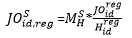
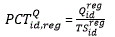
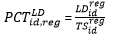
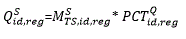
These estimates are based upon a model. BLS constructed a methodology to produce error measures of estimates, which will be updated annually.

Composite Synthetic Model

What approach?

The Composite Synthetic approach uses the Synthetic estimate in all state-supersector cells that have fewer than five respondents. In all state-supersector cells with
5–30 respondents an estimate is calculated that is a composition of a weighted estimate of the microdata-based estimate and a weighted estimate of the Synthetic estimate. The weight assigned to the JOLTS data in those cells is proportional the number of JOLTS respondents in the cell (weight=n∕30, where n is the number of respondents).

The Composite Synthetic supersector estimates are summed across state-supersectors to the nonfarm level.

What data inputs?

All JOLTS microdata records
All weights from JOLTS estimation (final weights that account for sampling weight, NRAF, agg-codes, etc.)
Synthetic estimates (regional JO, H, Q, LD, and TS rates)
JOLTS regional-level estimates (to benchmark the state estimates)
CES state-supersector employment

How are data used?

All JOLTS microdata are weighted using final weights. A weighted estimate is made for each JOLTS respondent.
Counts are made for each state-supersector cell.
Each JOLTS respondent is paired with its Synthetic rate estimate for all variables.
Based on the count of respondents in the state-supersector cell the JOLTS respondent belongs to, a Composite Model Weighted (CMW) estimate is calculated.

If the count is>30, then the CMW for the respondent data=1. The CMW for the Synthetic estimate=0.
If the count<5, then the CMW for the respondent data=0. The CMW for the Synthetic estimate=1.
If the count is 5–30, then the CMW for the respondent data=n∕30, where n is the number of respondents. The CMW for the Synthetic estimate=1−n∕30.

The state-level rate estimate is therefore the final weighted respondent-based JOLTS rate times the CMW added to the Synthetic rate times the CMW, benchmarked to CES state-level estimate:

FINAL ESTIMATE=CES STATE EMP×((final weight JOLTS rate×CMW)+(synthetic rate×CMW))

To stabilize the estimate, the sum of state Composite Synthetic estimates within each region is then benchmarked to the published JOLTS regional estimates.

How are outputs produced, and what are the limitations?

This model produces state-level estimates of JO, H, Q, LD, and TS. These estimates cannot be produced without lag.

What more is needed?

These estimates are based upon a model. BLS constructed a methodology to produce error measures of estimates, which will be updated annually.

Seasonal Adjustment

Most series published by the Job Opening and Labor Turnover Survey (JOLTS) program have a regularly recurring seasonal movement that can be measured from past data. Seasonal adjustment eliminates the component of the change attributable to the normal seasonal variation and makes it possible to observe the cyclical and other nonseasonal component movements in the series. The JOLTS program uses X-13-ARIMA-SEATS software developed by the U.S. Census Bureau to seasonally adjust the monthly estimates. The X-13-ARIMA-SEATS software is available on the U.S. Census Bureau website. The JOLTS program employs a concurrent seasonal adjustment methodology to seasonally adjust its estimates.

Seasonal adjustment input files

All controllable variables remain fixed during the year. For example, the ARIMA model, outliers, transformation specification, and historical data are held constant. Once a year, as part of the annual JOLTS benchmark procedure, all seasonal adjustment specifications are reviewed for each series. Any changes are implemented and kept constant until the next annual benchmark. Also during the annual benchmark, estimates for the 5 most recent years are readjusted using the new specifications. Estimates are only revised back for a 5-year period.

Additive and multiplicative models

The model specifications provide the mode (additive or multiplicative) selected for each JOLTS series by state. Depending on the relationship between the original series and each of the components, the mode of seasonal adjustment may be additive or multiplicative. Formal tests are conducted to determine the appropriate mode of adjustment.

The multiplicative mode assumes that the magnitude of the seasonal pattern is proportional to the level, which implies that the size of the seasonal fluctuations increases and decreases with the level of the series. With this mode, the monthly seasonal factors are ratios, with all positive values centered around one. The seasonally adjusted values are computed by dividing each month's original value by the corresponding seasonal factor.

In contrast, the additive mode assumes that the magnitude of the seasonal pattern is independent of the level of the series. In this case, the seasonal factors represent positive or negative deviations from the original series and are centered around zero. The seasonally adjusted values are computed by subtracting the corresponding seasonal factor from each month's original value.

Regional raking procedure

A raking procedure is used to ensure that the sum of the seasonally adjusted state series is consistent with the published seasonally adjusted total at the regional levels. The raking procedure begins by seasonally adjusting the regional and state level series independently. The seasonally adjusted state series are summed to the regional levels to get the regional totals. Ratios of seasonally adjusted state-to-regional levels are calculated. The regional totals summarized from the seasonally adjusted state series are subtracted from the official regional seasonally adjusted estimates to determine the amount that must be raked. The total amount that must be raked is multiplied by the ratios to determine what percentage of the raked amount should be applied to each state. Once the seasonally adjusted state series receive their proportional amount of the raked values, the two groups are aggregated again to regional totals. At this point their sum should be equal to the official regional seasonally adjusted estimate.

Sample Allocation

What is the sample size allocation for the inputs used to produce the JOLTS state estimates?

The JOLTS state estimates sample allocation table below provides a snapshot of the sample used to produce December 2024 and December 2025 state estimates. Sample are utilized in both components of the model. The sample component table includes JOLTS state respondent and sample data. The model component includes JOLTS regional-level sample and respondent data, CES state respondent data, and QCEW establishment counts.

SAMPLE ALLOCATION: For State Estimator Components
State	FIPS Code	Region	JOLTS State Sample ^[1]		JOLTS State Respondents^[2]		JOLTS Regional-level Sample^[1]		JOLTS Regional-level Respondents^[3]		QCEW Establishments^[4]		CES State^[5]
State	FIPS Code	Region	2024	2025	2024	2025	2024	2025	2024	2025	2024	2025	2024	2025
Alabama	1	South	329	338	98	105	8,599	8,763	2,183	2,186	158,900	163,959	13,060	12,130
Alaska	2	West	87	82	28	31	6,733	6,666	1,581	1,515	24,987	25,004	2,250	2,240
Arizona	4	West	589	597	144	136	6,733	6,666	1,581	1,515	217,387	219,716	12,520	11,520
Arkansas	5	South	173	192	54	63	8,599	8,763	2,183	2,186	103,802	110,271	6,580	6,200
California	6	West	3,208	3,129	654	616	6,733	6,666	1,581	1,515	1,900,725	2,003,227	67,560	66,670
Colorado	8	West	593	578	172	155	6,733	6,666	1,581	1,515	235,253	256,470	9,740	9,720
Connecticut	9	Northeast	341	341	100	88	6,040	6,049	1,550	1,499	145,568	145,755	6,560	6,140
Delaware	10	South	64	68	21	21	8,599	8,763	2,183	2,186	43,367	45,414	1,970	2,030
District of Columbia	11	South	113	112	21	24	8,599	8,763	2,183	2,186	50,093	48,967	2,070	1,940
Florida	12	South	1,528	1,554	332	365	8,599	8,763	2,183	2,186	885,078	859,789	38,580	41,180
Georgia	13	South	711	712	192	181	8,599	8,763	2,183	2,186	384,071	387,688	24,910	24,160
Hawaii	15	West	102	95	19	21	6,733	6,666	1,581	1,515	58,036	59,596	2,220	2,340
Idaho	16	West	176	172	54	45	6,733	6,666	1,581	1,515	100,258	101,159	4,270	4,150
Illinois	17	Midwest	1,255	1,238	308	292	6,343	6,290	1,679	1,670	391,565	386,281	19,920	18,850
Indiana	18	Midwest	586	562	155	153	6,343	6,290	1,679	1,670	190,190	191,491	11,410	10,670
Iowa	19	Midwest	284	273	85	84	6,343	6,290	1,679	1,670	111,148	109,859	8,760	8,250
Kansas	20	Midwest	330	329	97	108	6,343	6,290	1,679	1,670	91,845	99,220	6,830	6,650
Kentucky	21	South	267	264	72	67	8,599	8,763	2,183	2,186	154,999	157,638	8,030	7,620
Louisiana	22	South	293	288	81	83	8,599	8,763	2,183	2,186	147,508	149,477	9,580	9,140
Maine	23	Northeast	150	143	49	40	6,040	6,049	1,550	1,499	64,252	65,694	4,780	4,400
Maryland	24	South	384	433	92	114	8,599	8,763	2,183	2,186	190,426	192,902	9,450	9,440
Massachusetts	25	Northeast	777	771	191	172	6,040	6,049	1,550	1,499	286,373	294,397	11,750	10,890
Michigan	26	Midwest	888	898	218	212	6,343	6,290	1,679	1,670	299,061	313,073	14,710	13,950
Minnesota	27	Midwest	525	543	147	149	6,343	6,290	1,679	1,670	214,600	214,802	8,960	8,920
Mississippi	28	South	192	199	65	62	8,599	8,763	2,183	2,186	87,224	88,129	6,650	6,420
Missouri	29	Midwest	622	597	154	151	6,343	6,290	1,679	1,670	249,924	257,215	15,070	14,800
Montana	30	West	137	130	31	37	6,733	6,666	1,581	1,515	64,723	61,545	3,510	3,600
Nebraska	31	Midwest	203	203	56	63	6,343	6,290	1,679	1,670	77,800	78,385	4,900	4,930
Nevada	32	West	231	245	53	62	6,733	6,666	1,581	1,515	107,909	110,722	3,650	3,580
New Hampshire	33	Northeast	174	179	55	50	6,040	6,049	1,550	1,499	67,075	66,039	4,200	4,480
New Jersey	34	Northeast	980	978	257	264	6,040	6,049	1,550	1,499	338,666	342,656	17,200	16,110
New Mexico	35	West	210	226	57	62	6,733	6,666	1,581	1,515	68,475	69,296	6,360	6,100
New York	36	Northeast	2,077	2,047	481	473	6,040	6,049	1,550	1,499	691,008	698,545	38,830	44,600
North Carolina	37	South	748	761	208	192	8,599	8,763	2,183	2,186	373,501	381,116	19,730	19,280
North Dakota	38	Midwest	153	147	45	41	6,343	6,290	1,679	1,670	35,820	36,145	2,720	2,470
Ohio	39	Midwest	965	961	265	263	6,343	6,290	1,679	1,670	345,616	347,848	23,970	23,670
Oklahoma	40	South	267	272	83	88	8,599	8,763	2,183	2,186	126,015	126,880	8,930	8,340
Oregon	41	West	327	329	91	89	6,733	6,666	1,581	1,515	180,576	170,922	11,850	12,570
Pennsylvania	42	Northeast	1,334	1,373	356	348	6,040	6,049	1,550	1,499	394,471	397,503	21,430	20,230
Rhode Island	44	Northeast	132	138	35	41	6,040	6,049	1,550	1,499	48,339	48,629	1,820	1,900
South Carolina	45	South	371	362	94	94	8,599	8,763	2,183	2,186	190,497	188,510	10,040	9,410
South Dakota	46	Midwest	86	92	31	31	6,343	6,290	1,679	1,670	40,503	40,855	2,450	2,420
Tennessee	47	South	443	463	130	111	8,599	8,763	2,183	2,186	225,321	214,749	12,920	12,160
Texas	48	South	2,014	2,042	463	453	8,599	8,763	2,183	2,186	836,955	851,439	49,820	49,700
Utah	49	West	368	358	98	86	6,733	6,666	1,581	1,515	141,514	143,636	7,550	6,960
Vermont	50	Northeast	75	79	26	23	6,040	6,049	1,550	1,499	33,195	33,991	2,180	2,200
Virginia	51	South	571	582	134	125	8,599	8,763	2,183	2,186	314,526	317,425	17,940	17,640
Washington	53	West	618	623	154	143	6,733	6,666	1,581	1,515	233,366	233,678	11,540	11,050
West Virginia	54	South	131	121	43	38	8,599	8,763	2,183	2,186	60,527	60,898	5,800	5,480
Wisconsin	55	Midwest	446	447	118	123	6,343	6,290	1,679	1,670	208,268	210,375	11,010	10,410
Wyoming	56	West	87	102	26	32	6,733	6,666	1,581	1,515	30,557	30,877	2,540	2,620
All states and D.C.			27,715	27,768	6,993	6,870	364,188	365,550	91,762	90,388	12,021,863	12,209,857	631,080	622,330
Footnotes: 1)JOLTS State and Regional - Level Sample 2)JOLTS Sample Units used in Sample Component of the Composite Model 3)JOLTS Sample Units used in Model Component of the Composite Model; the Total is the sum of the four regions 4)QCEW Establishments used in the Model Component of the Synthetic and Composite Synthetic Model 5)CES UI Sample Units used in Model Component of the Composite Synthetic Model

Reliability of Estimates

What is the reliability of the JOLTS state estimates?

JOLTS state estimates are subject to both sampling and nonsampling error. Sampling error occurs when a sample is surveyed rather than the entire population. There is a chance that the sample estimates may differ from the true population values they represent. The difference, or sampling error, varies depending on the particular sample selected. This variability is measured by the standard error of the estimate. BLS analysis is generally conducted at the 90-percent level of confidence. That means that there is a 90-percent chance, or level of confidence, that an estimate based on a sample will differ by no more than 1.6 standard errors from the true population value because of sampling error.

The JOLTS state estimates also are affected by nonsampling error. Nonsampling error can occur for many reasons including: the failure to include a segment of the population; the inability to obtain data from all units in the sample; the inability or unwillingness of respondents to provide data on a timely basis; mistakes made by respondents; errors made in the collection or processing of the data; and errors from the employment benchmark data used in estimation.

The JOLTS State variance estimates account for both sampling error and the error attributable to modeling. A small area domain model uses a Bayesian model to develop estimates of JOLTS State variance. The small area model uses QCEW-based JOLTS synthetic model data to generate a Bayesian prior distribution, then updates the prior distribution using JOLTS microdata and sample-based variance estimates at the State and US Census Regional level to generate a Bayesian posterior distribution. Once the Bayesian posterior distribution has been generated, an estimate of JOLTS State variance estimates is made by drawing 2,500 estimates from the Bayesian posterior distribution. This Bayesian approach thus indirectly accounts for sampling error and directly for model error. The median standard errors table by state is available on the JOLTS Median Standard Errors page. The error measures will be updated annually.

Last Modified Date: July 23, 2026