
An official website of the United States government
An official website of the United States government
The .gov means it's official.
Federal government websites often end in .gov or .mil. Before sharing sensitive information,
make sure you're on a federal government site.
The site is secure.
The
https:// ensures that you are connecting to the official website and that any
information you provide is encrypted and transmitted securely.
This is an archived page. To see the latest version, please visit Employment Projections: Calculation.
Over the years, the U.S. Bureau of Labor Statistics (BLS) has undertaken many changes in its employment projections as new data series became available and as economic and statistical tools improved. Since the late 1970s, however, the basic methodology has remained largely the same. Procedures have centered on: projections of an interindustry, or input–output, model that determines job requirements associated with production needs, and the National Employment Matrix, which depicts the distribution of employment by industry and occupation. Projecting employment in industry and occupational detail requires projections of the total economy and its sectors. BLS develops its 10-year projections in a series of six steps that examine:
Each step is based on separate procedures, models, and related assumptions. All steps go through several iterations to ensure an internal consistency of results. The results are reviewed and revised with each iteration. If necessary, relevant assumptions may be revised. Together, the six components provide the analytical framework needed to develop detailed employment projections. BLS analysts solve these six components sequentially.
Projections of the future supply of labor are calculated by applying BLS labor force participation rate projections to population projections produced by the Census Bureau. The Census Bureau carries out long-term projections of the resident U.S. population. The projection of the resident population is based on the current size and composition of the population and includes assumptions about future fertility, mortality, and net international migration. BLS analysts then convert the resident population concept of the decennial census to the civilian noninstitutional population concept of the BLS Current Population Survey (CPS). This takes place in three steps. First, the population of children under age 16 is subtracted from the total resident population. Then, the population of the Armed Forces, by age, gender, race, and ethnic categories, is subtracted out. Finally, the institutional population is subtracted from the civilian population for all the different categories.
BLS maintains a database of annual averages of labor force participation rates provided by CPS for various age, gender, race and ethnic groups. BLS analysts examine trends and the past behavior of participation rates for each of the categories. This is accomplished by first smoothing the historical participation rates for these groups. Next the smoothed data are transformed into logits, or the natural logarithm of the odds ratio.1 Then, the logits of the participation rates are extrapolated linearly by regressing them against time and then extending the fitted series to or beyond the target year. When the series are transformed back into participation rates, the final projected paths are nonlinear.
In addition, projected labor force participation rates are reviewed for consistency. Reviews are conducted on the time path, the cross section in the target year, and the cohort patterns of participation, and, if necessary, modifications are made. Projected labor force participation rates are then applied to the projected civilian noninstitutional population, producing labor force projections for each of the age, gender, race, and ethnic groups. Finally, these groups’ values are summed to obtain the total civilian labor force, a key input into projecting the macroeconomy, which is the next step.
The second stage of the BLS projections process develops projections of the macroeconomy. Values projected include gross domestic product (GDP) for the United States and the major categories of demand and income. The results of this stage provide aggregate measures that are consistent with each other and with the various assumptions and conditions of the projections. Values generated for each demand sector are then used in the next stage: developing data on detailed commodity purchases for personal consumption, business investment, foreign trade, and government.
Recent projections are produced by using the US Macro Model, licensed from Macroeconomic Advisers by IHS Markit (MA). Prior to the 2012–22 projections, BLS relied on MA’s Washington University Macro Model (WUMM). MA/US has the same foundations as WUMM: consumption follows a life-cycle model and investment is based on a neoclassical model. Foreign sector estimates rely on forecasts from Oxford Economics. The MA/US model is explicitly designed to reach a full-employment solution in the target years, which is consistent with the BLS long-run view of the economy. In a full-employment economy, any unemployment is frictional and is not a consequence of deficient demand. Within MA/US, a submodel calculates an estimate of potential output from the nonfarm business sector, based upon full-employment estimates of the sector’s hours worked and output per hour. Error correction models are embedded into MA/US to align the model’s solution with the full-employment submodel.
The BLS projections depend on underlying assumptions about the future. Because the projections are used for career planning, training and education, and policy planning, structural changes are more important than cyclical changes. The full employment assumption allows for an analytical focus on structural changes to the economy rather than the cyclical deviations of the business cycle. BLS defines full employment as an economy in which the unemployment rate equals the nonaccelerating inflation rate of unemployment (NAIRU), no cyclical unemployment exists, and GDP is at potential given available resources. The full employment assumption gives users an objective expectation that the projected levels of employment and output are consistent with the economy approximately at the peak of the business cycle. Projections efforts should always be considered subject to revision as new information becomes available. Since projections are consistently benchmarked to this same objective level, users are provided a means to evaluate both prior and current projections to interpret the data in a way that is best for them.
Certain critical variables set the parameters for the nation’s economic growth and determine, in large part, the trend that GDP will follow. In developing the macroeconomic projections, BLS elects to determine these critical variables externally through research and modeling, and then supplies them to the MA/US model as exogenous variables. The in-house labor force projections, described above, are of particular importance as they are the primary constraint on future economic growth. Other fundamental exogenous variables in the model include energy prices and assumptions about fiscal and monetary policy.
Besides being governed by general assumptions, projections are also assessed on their economic validity. Economic concepts that are assessed include the rate of growth and demand composition of real GDP, the rate of growth of labor productivity, the rate of inflation, and the unemployment rate. Many iterations may be necessary to arrive at a balanced set of assumptions that yield a defensible set of results. When the aggregate economic projection is final, the components of GDP are supplied to the commodity component of the projections process. These components of GDP include consumer expenditure, investment, changes in private inventories, exports, imports, and government spending.
The macroeconomic model provides projections of final demand sectors, including personal consumption expenditures (PCE), private investment in equipment (PEQ), private investment in intellectual property products (IPP), residential and nonresidential structures, changes in private inventories (CIPI), exports and imports of goods and services, and consumption and investment of federal and state and local governments. The next step in the projections process is to further disaggregate these results into detailed categories and then into the types of commodities purchased within each category. The sectoring plan is chosen to be as detailed as possible only to the extent that categories and commodities are supported by the national income and product accounts (NIPA) and the input–output accounts, both published by the Bureau of Economic Analysis (BEA).2
The Houthakker-Taylor model is used to estimate consumption expenditures for 78 detailed product categories over the projection period.3 Consumption of each product type is modeled on the basis of its historical relationship with disposable income, prices, and a state variable capturing inventory or habit formation. Likewise, investment is modeled for 32 asset categories (29 for PEQ, 3 for IPP) using the Modified Neoclassical model, wherein investment is determined by GDP, capital stock, and the rental cost of capital. Next, the PCE and investment category estimates are chain weighted to their aggregate levels and adjusted as necessary to ensure consistency with the macroeconomic model solution.4
The controls for nonresidential and residential structures, exports and imports of goods and services, as well as consumption and investment within federal defense, federal nondefense, and state and local government are supplied directly from the macro model. Slight adjustments are made to the model’s breakout of net exports to account for re-exports and re-imports, effectively revising the data from a NIPA-based estimate to an input–output definition.
Once the column totals for consumption, investment, government, and trade are projected, a bridge table is developed based on historical relationships within the input–output accounts. The bridge table is used to distribute the projected total for each demand category among 205 commodities.
Business inventories are extrapolated at the commodity level of detail using a two-stage least squares model where inventories are regressed on lagged values of both inventories and commodity output. Detailed projections of inventories are then aggregated and adjusted to conform to the macroeconomic model solution.
Other factors are then considered in adjusting initial distributional relationships. For example, the trade outlook may consider research such as external energy forecasts, existing and expected shares of the domestic market, expected world economic conditions, and known trade agreements. The relationship among commodities for government categories may factor in analysis including current trends in spending patterns as well as expectations of government policy changes.
As a last step, data are converted from purchaser value to producer value. Margin columns are projected for each component of final demand based upon distributional relationships from the historical time series. Summing across the rows of a particular component with its related margin columns (consisting of transportation costs as well as wholesale and retail markups), results in a vector of producer value data by detailed commodity. Producer value data are important to the employment projections, as they separate output and therefore the job outlook in the wholesale, retail, and transportation industries apart from the remaining economy.
For a simplified example of producer value data for one commodity, see table 1. To track the purchase of a sweater, for example, an analyst would first measure the transaction as a purchaser value in column A. The customer paid $20 for the sweater, which is allocated entirely to the textile row. Column B shows the retail trade markup value for the sweater. The retailer in this case marked up the sweater by $10 as captured by a negative value in the textile row and an equivalent positive value in the retail trade row. The margin column is just reallocating data and therefore sums to zero. The producer value of this same transaction is shown in column C, the row sum of columns A and B. The producer value for this purchase is $10 for textile commodity and $10 for retail trade. The summed value of the purchaser and producer value columns are equivalent.
| Commodity rows | A | B | C |
|---|---|---|---|
| Consumption of clothing | Retail trade | Consumption of clothing | |
| Textiles | $20 | –$10 | $10 |
| Other goods | 0 | 0 | 0 |
| Retail trade | 0 | $10 | $10 |
| Services | 0 | 0 | 0 |
| Remaining commodities | 0 | 0 | 0 |
| Sum | $20 | 0 | $20 |
The components of final demand and the margin columns are compiled into a final-demand matrix comprising 205 rows of commodity sectors and 153 columns of final-demand and margin categories.5 The resulting detailed distribution of GDP provides the demand component of an interindustry model of the U.S. economy.
The creation of an input–output model is the next stage in developing BLS projections.6 Each industry within the economy relies on other industries to supply inputs—intermediate products or services—for further processing. By definition, GDP reflects only sales to final purchasers, such as car buyers for personal use and businesses for equipment. Intermediate material inputs, such as the steel incorporated into cars, are not explicitly reflected in the GDP estimates. An input–output model provides a means to derive an industry-level estimate of the output and employment needed to produce a given level of GDP. The number of rows and columns, or sectors, in an input–output system determines the level of industry detail. The BLS sector plan, based on the North American Industry Classification System (NAICS), has 205 sectors.
BLS develops a historical time series of input–output tables. In the past, this has been accomplished through the use of various source data from a number of different data providers, including the Bureau of Economic Analysis (BEA), Census Bureau, U.S. Department of Agriculture, U.S. Energy Information Administration, U.S. Geological Survey, and various other ancillary information sources. These data were compiled, and, using the most current BEA benchmark input–output accounts as the basis, BLS developed historic input–output tables.
Starting with the 2010–20 projections series, BLS changed its methods of developing historic input–output. The change was prompted by the BEA publication in 2009 of a comprehensive revision to its input–output framework. The BEA revision reinstituted publication of annual input–output data and established a standardized and consistent framework between the more detailed benchmark input–output data and the more aggregated annual input–output systems. Using both the 1997 and 2002 benchmark input–output tables as the basis, scaling the detailed BEA benchmark tables to the BLS sector plan, and making adjustments conforming to BLS assumptions and methods, BLS used the scaled benchmark BEA tables to create pattern structures to develop the detailed sector input–output tables for non-benchmark years. Under this methodology, and based on the pattern structures developed from the scaled benchmarks, the BEA annual input–output tables (which feature much less detail than the benchmarks) were expanded. The years between the two benchmarks included interpolation factors to accommodate changes to the patterns between the benchmark years while patterns for later years were held constant from the most timely benchmark table. After all of the tables were developed under the BLS sector plan, each table was RAS balanced (iteratively scaled) to ensure consistency, conformity, and equality.7 In 2014, BEA published another comprehensive revision that included a 2007 benchmark table and also achieved greater consistency between the annual and benchmark tables. In 2018, BEA conducted another comprehensive revision that was based on the 2012 NAICS, and included updates to the 1997, 2002, and 2007 benchmark tables and a new release for the 2012 benchmark input-output table. Additionally, the 1997–2017 annual tables were revised to be consistent with the benchmark input-output tables. As was done previously, interpolation factors between benchmark years, 1997–2002, 2002–07, and 2007–12, were developed and used to expand the annual input–output tables to the BLS sector plan. For years after the 2012 benchmark, the pattern structure for 2012 was used to expand the annual tables.
The BLS input–output model consists of two basic matrices for each year: a “use” table and a “make” table. Once balanced, both tables are converted to coefficient form. The converted “use” table, or the direct requirements table, shows the use of commodities by each industry as inputs into its production process. Each column of this table displays the pattern of commodity inputs per dollar of industry output. The converted “make” table, or the market share table, shows the commodity output of each industry. This table allocates commodity output to the industry in which it is the primary commodity output and to those industries in which it is secondary. The “make” table also shows the industry distribution of production for each commodity. Initial estimates of the projected input–output tables are based on historical relationships and the projected final demand tables. Results are then reviewed and revised in order to take into account changing trends in the input patterns, or the way in which goods are produced or services provided by each industry.
When projected values of the “use” and “make” relationships are available, BLS uses the relationships derived by BEA to convert the projection of commodity demand developed in preceding steps into a projection of domestic industry output. The BEA relationships are summarized in the formula:
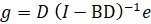
where:
g = vector of domestic industry output by sector
B = “use” table in coefficient form
D = “make” table in coefficient form
I = identity matrix
e = vector of final demand by commodity sector
In sum, the matrix product of the inverse of the coefficient forms of the “make” and “use” tables and a vector e of final demand commodity distribution yields industry outputs.
The detailed industry output from the previous stage is used to derive the industry employment estimate necessary to produce the given level of output. To arrive at the employment estimate, the Employment Projections (EP) program combines data from two BLS sources: (1) the Current Employment Statistics (CES) survey, an establishment survey that offers data on nonagricultural wage and salary employment and weekly hours and (2) the Current Population Survey (CPS), a household survey that provides information regarding agricultural employment, self-employed workers and hours, and private household workers.
The data provided by CES are measurements of the number of jobs. The data provided by CPS are measurements of the number of people. This distinction matters as individuals may hold more than one job. The CES data are the principal source of historical employment data for the projections program. However, the CES data only cover nonfarm payroll jobs and do not include agricultural sector, private household, or self-employed workers. The CPS data are used to supplement CES where data would otherwise not be available. The projections program uses the CPS person-based measure of employment in a manner that assumes one job per person. In the remainder of this section, references to workers should be understood as a reference to a single job.
Many assumptions underlie the BLS projections of the aggregate economy and of industry output, productivity, and employment. Often, these assumptions bear specifically on econometric factors, such as the aggregate unemployment rate, the anticipated time path of labor productivity, and expectations regarding the Federal budget surplus or deficit. Other assumptions deal with factors that affect industry-specific measures of economic activity.
BLS models industry employment as a function of industry output, wages, prices, and time. BLS projects industry employment, using the estimated historical relationship between these variables. Industry employment is projected in both numbers of jobs and hours worked, for wage and salary jobs and for self-employed workers. Projections are developed according to the procedure outlined next, implemented for each industry.
A system of equations projecting employment for wage and salary jobs is solved independently over the projections decade for each industry. The individual industry estimates of employment must be consistent with the total level of employment derived from the solution of the macroeconomic model. The employment equations relate an industry’s labor demand (total hours) to its output, its wage rate relative to its output price, and a trend variable in order to capture technological change within that industry. A separate set of equations, describing average weekly hours for each industry, is estimated as a function of time and the unemployment rate. The two sets of equations are then used to predict average weekly hours over the projections decade. An identity relating average weekly hours, total hours, and employment yields a count of wage and salary jobs by industry.
The number of self-employed workers is derived by first extrapolating the ratio of the self-employed to the total employment for each industry. The resulting extrapolation is a function of time and the unemployment rate. The extrapolated ratio is used to derive the number of self-employed workers, given the number of wage and salary jobs in each industry. Total hours for self-employed workers are calculated by applying the estimated number of annual average weekly hours to the employment levels for each industry. Finally, total hours for each industry are derived by summing hours for wage and salary jobs and hours for self-employed workers.
Together with industry output projections, employment results provide a measure of labor productivity. BLS analysts examine the implied growth rates in the projected productivity numbers for consistency with historical trends. At the same time, analysts attempt to identify industries that may deviate from past behavior because of changes in technology or other factors. Where appropriate, changes to the implied productivity are made by modifying the employment demand. The final estimates of projected employment for about 200 industries are then used as inputs to determine the occupational employment over the projections decade.
BLS creates occupational employment projections in a product called the National Employment Matrix. This matrix describes the employment of detailed occupations within detailed wage and salary industries and different classes of workers, including those who are self-employed or employed by a private household. The matrix provides a comprehensive count of nonfarm wage and salary jobs—which is different from a count of workers, since a single worker may hold more than one job—and a count of self-employed workers, agricultural industry workers, and workers employed in private households. These counts are provided for a base year and a projected year, which is 10 years in the future.
The matrix does not include employment for every possible combination of industry and occupation. Some data are not released to protect the confidentiality of the businesses or individuals providing the data and others are not released for quality reasons. All employment data in the National Employment Matrix are presented in thousands, rounded to one decimal place. The detailed data in the matrix may not sum to summaries because of rounding or data that are not released.
The coverage of the National Employment Matrix can be divided into two groups:
Nonfarm wage and salary employment is by far the larger of the two groups. These jobs are grouped into industries and occupations that generally match those released in the OES data. The data used in the matrix to describe the base year for these jobs come from three sources. Job counts by industry come from CES, which covers nonfarm payroll jobs. In places where the matrix is more detailed than CES industry data, the QCEW is used to develop weights to provide further detail. Industry employment is split into individual occupations using OES data that describe what share of industry employment is held by which occupations.
Self-employed workers, workers employed by private households, and agricultural workers (excluding the logging industry) account for a small share of total employment. Because these workers are not captured by establishment survey programs like OES and CES, the matrix uses data from CPS, which is a household survey that collects data directly from the workers. As a result of collecting data from workers, CPS data used by the matrix are a count of workers, not jobs, which is different from the measure used for nonfarm wage and salary jobs.
One additional note on matrix use of CPS data: CPS data are coded using the Census Occupation Classification System, which has fewer, broader occupations than the Standard Occupational Classification (SOC) system. Both OES and the National Employment Matrix use SOC. To make CPS occupational data comparable with SOC, OES occupational data are applied as weights to divide CPS occupations into the more detailed SOC occupations.
Projected-year employment data for wage and salary jobs, including all agricultural workers, and workers employed by private households are developed using a conceptual framework that divides industry employment between occupations based on expected, structural changes in the demand for those occupations within a given industry. To project these changes in occupational demand, BLS economists thoroughly review qualitative sources such as articles, expert interviews, and news stories, as well as quantitative resources such as historical data and externally produced projections. These reviews identify structural changes in the economy which are expected to change an occupation's share of industry employment.
The sum of shares of industry employment for all the occupations in an industry must add up to 100 percent for the occupational employment within an industry to match the overall industry's projected employment. As a result, changes to one or more occupations' shares of industry can scale the shares of other occupations in that industry. To prevent unintended changes, the scaled shares of industry employment are reviewed extensively to ensure that changes in each industry are consistent with each other and that individual changes support the broader industry's narrative and projection.
Each occupation in the matrix is analyzed to identify factors that are likely to cause an increase or decrease in demand for that occupation within particular industries. This analysis incorporates judgments about new trends that may influence occupational demand, such as expanding use of new manufacturing techniques like 3D printing that might change the productivity of particular manufacturing occupations, or shifts in customer preferences between different building materials that may affect demand for specific construction occupations.
Among the various factors that can affect the demand for an occupation in an industry are:
The results of this qualitative analysis form the quantitative basis for making changes to occupational shares of industry employment. The structural changes suggested by different trends are compared to determine if they will cause demand to grow or shrink, and if so, by how much. The effects of the projected trends are then combined into an overall numerical estimate which describes the change in an occupation's share of industry employment.
Projected-year data for self-employment are created using a modified version of the wage and salary employment method. Wage and salary employment is analyzed at an occupation-by-industry level but self-employment data at that same level result in estimates which are too small to analyze reliably. Additional difficulties finding sufficient qualitative information about self-employment by occupation and industry make analysis at this level impractical even if robust data were available.
To provide more usable estimates, self-employment data are initially projected at the occupation-by-industry level but aggregated to the occupational level for analysis. That is, the details about individual occupations in specific industries for self-employed workers are combined to show the growth or decline of self-employed workers overall for each occupation. Although this broader view of self-employed workers does not provide the same detail as wage and salary, the rate of growth or decline for self-employed occupations does incorporate the underlying industry detail, providing a reasonable estimate for analysis. As with other CPS occupational data, these estimates are based on the Census Occupation Classification System, and the matrix uses OES employment data as weights to provide the more detailed SOC structure for analysis and publishing.
The methods used for wage and salary and self-employed worker projections are similar in their reliance on qualitative and quantitative research. Both examine available data and other resources. Both make changes when the information available suggests a structural change is happening or is likely to occur before the projected year. Both incorporate changing industry demand for the occupation, but self-employment projections do this at a less detailed level than wage and salary.
Projections of job growth provide valuable insight into future employment opportunities because each new job created is an opening for a worker entering an occupation. However, opportunities also arise when workers separate from their occupations and need to be replaced. In most occupations, occupational separations provide many more openings than employment growth does.
To project the magnitude of occupational openings, BLS calculates an estimate of the number of workers expected to exit the labor force, due to retirement or other factors, and an estimate of the number of workers expected to transfer to a different occupation. The sum of labor force exits and occupational transfers represents the total projected separations for each occupation. This estimate does not count workers who change jobs but remain in the same occupation.
To develop estimates of separations, BLS uses two separate calculations based on data from the Current Population Survey (CPS), a household survey that collects demographic and employment information about individuals. In the first calculation, data from the monthly CPS are used to estimate a regression model that measures the propensity of workers to exit the labor force. In the second, data from the CPS Annual Social and Economic Supplement (ASEC) are used to estimate a regression model that measures the propensity of workers to transfer to a different occupation. Both models are estimated using worker demographics and job specific information as independent variables.
The results of the regression models are applied to the current demographics of each detailed occupation to estimate the propensity of current workers to separate from the occupation. This is used to generate a projected labor force exit rate and an occupational transfer rate for each occupation, which is applied to the projected level of employment to calculate the number of separations projected for an occupation. Occupational separations can then be added to the projected employment change in an occupation to identify the total occupational openings available for new workers to enter.
The CPS data used to calculate separation rates are coded in accordance with the Census Occupation Classification System. The occupational employment projections use occupational codes from the Standard Occupational Classification (SOC) system, which are often more detailed than the U.S. Census Bureau's occupational classifications. To apply CPS data to the occupations in the projections matrix, BLS identifies the CPS occupations that are equivalent to, or that included, a given detailed SOC occupation.
BLS also provides information about education and training requirements for each of the occupations for which it publishes projections data. This approach allows occupations to be grouped in order to create estimates of the outlook for occupations with various types of education or training needs. In addition, educational attainment data for each occupation are presented to show the level of education achieved by current workers.8
An important element of the projection system is its comprehensive structure. To ensure internal consistency and reasonableness of this large structure, the BLS projections process encompasses detailed reviews and analyses of the results at each stage. For example, the close relationship between changes in staffing patterns in the occupational model to changes in technology is an important factor in determining industry labor productivity. Specialists in many different areas from inside and outside the BLS projections group review all of the relevant results from their particular perspective. In short, final results reflect innumerable interactions among BLS analysts, who focus on particular sectors in the model. Through this review, the projection process at BLS converges into an internally consistent set of employment projections across all industries and occupations.
BLS employment projections are developed with a number of underlying assumptions, both explicit and implicit. Projections are developed from statistical and econometric models combined with subjective analysis. All analytical projections implicitly assume that relationships exhibited in the past will continue to hold over the projection period. Statistical and econometric models formally project historical relationships on a mathematical basis. Subjective analysis projects current and historical behavior into the future on the basis of analogous past experience. The efficacy of the projections relies both on the understanding of history and the expectation that the past can be extrapolated into the future.