An official website of the United States government
An official website of the United States government
The .gov means it's official.
Federal government websites often end in .gov or .mil. Before sharing sensitive information,
make sure you're on a federal government site.
The site is secure.
The
https:// ensures that you are connecting to the official website and that any
information you provide is encrypted and transmitted securely.
The Office of Productivity and Technology (OPT) produces measures of productivity for the entire economy at various levels of aggregation, including the six major industry sectors in the United States: business, nonfarm business, nonfinancial corporations, total manufacturing, durable goods manufacturing, and nondurable goods manufacturing. OPT also produces estimates of national productivity growth for detailed industries and estimates of aggregate productivity growth for states and regions. OPT compiles and analyzes a wide array of data produced by government statistical agencies and non-governmental organizations to measure productivity.
Productivity statistics measure how efficiently economic inputs are converted into output. The two primary productivity measures that the U.S. Bureau of Labor Statistics (BLS) produces are laborproductivity and totalfactorproductivity. In addition to these measures, BLS produces productivity measures based on other inputs, such as capital productivity.
To construct the measures of output and combined inputs used for productivity calculations, BLS uses the chained Törnqvist index number formula. The units of inputs vary (e.g. hours of work or tons of coal), so each one is converted to a growth rate and these are combined. Indexes represent the relative change in quantities and can be used to calculate the combined changes in inputs with different units, weighted by average cost shares of each input. Similarly, indexes can be used to aggregate different products to construct output for different sectors of the economy using average value shares as weights.
An index can be chained by multiplying, period-by-period, indexes calculated from underlying data for each consecutive pair of periods. The chain makes it possible to compare quantity indexes in any two periods. Chaining connects the changes from period b, the base period, to any period t. The indexes used in BLS productivity calculations are chained, and the index is set to have the value 100 in the base period b.
A Törnqvist index summarizes change over time in an economic aggregate. The Törnqvist index for each pair of periods is a link in the chain that makes up a chained Törnqvist index. It is calculated as a geometric mean of the relative change in quantities in time t from those in the preceding period t − 1. The relative changes in the quantities (products or inputs) are weighted using an average value or cost share in the two periods. For example, a Törnqvist index for output, Q, is calculated by aggregating n products, with quantities q, from two periods, using the following formula:
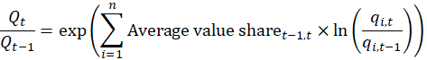
where

pi,t = price of product i at time t, and pi is the vector of all n prices at time t.
For simplicity, we often denote such a quantity index using notation such as:

Labor productivity (LP), or output per hour, is the efficiency with which output is produced via labor hours. Labor productivity is the ratio of real output to total hours worked, with output produced and hours worked measured per quarter or per year.

where real output is real value-added output for large sectors, such as nonfarm business, and real sectoral output for manufacturing sectors and detailed industries.
BLS publishes estimates of annual labor productivity growth rates where t is a year, which are calculated as:
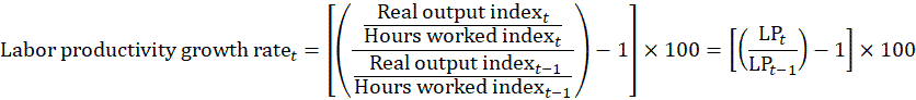
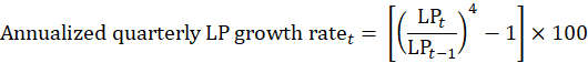
Quarterly estimates of labor productivity growth are expressed at an annual rate (as if the quarterly growth rate continued for a full year) where t is a quarter as follows:
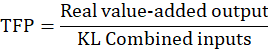
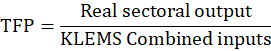
Total factor productivity (TFP) is the efficiency at which combined inputs are used to produce output. BLS produces value-added TFP for major sectors of the economy. Value-added TFP is the ratio of real value-added output to combined inputs, where inputs are capital (K) and labor (L).
BLS also produces sectoral output TFP (known as KLEMS TFP) for industries, where KLEMS stands for capital (K), labor (L), energy (E), materials (M), and services (S). Sectoral output TFP is calculated as the ratio of real sectoral output to combined inputs, where inputs are capital, labor, energy, materials, and services:
Output is the amount of goods and services produced. This section explains how to calculate sectoral output, real sectoral output, and value-added output.
Sectoral output is the current dollar value of goods and services produced by an industry for delivery to consumers outside that industry. Sectoral output measures are used to estimate annual productivity growth for North American Industry Classification System (NAICS) industries. At the industry level, sectoral output is calculated as the current dollar value of shipments plus the current dollar change in inventories minus the current dollar resales minus the current dollar intra-industry shipments. Sectoral output also represents the amount of capital, labor, energy, material, and service purchases an industry has used in production.


Real sectoral output is the amount of goods and services produced by an industry for delivery to consumers outside that industry. Aggregating from either the product line or from the industry, real sectoral output is calculated as a chained value-share-weighted Törnqvist index of either product line items or industry output. Product line items and industry output are adjusted to avoid double counting of output during aggregation. Real sectoral output is usually calculated by deflating product lines by price indexes but is sometimes computed using physical quantity levels.

For sectoral production based on industry aggregation, real sectoral output is calculated as a chained value-share-weighted Törnqvist index of component industry output. Sectoral output is adjusted to avoid double counting of output during aggregation:

Value-added output is a more narrowly defined concept of output that removes the value of purchased intermediate inputs of energy, materials, and services inputs from the value of sectoral output. Value-added output for the aggregate economy (GDP) equals the sum of value-added outputs of component industries. It can also be measured as the value of goods and services that are sold to final consumers. Value-added output reflects the contributions of primary inputs to production, capital and labor, which add value as intermediates are transformed into output.
This section explains how to calculate the labor hours worked that are used to produce labor productivity measures. It also explains how to measure labor input used in TFP measures that include an adjustment for the education and experience of the workforce.
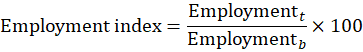
Employment is measured as the number of jobs in a given sector. An individual who works multiple jobs has each of their jobs counted in the measure of employment, which is a count of jobs, not people. The workers included in the employment measure may consist of either (1) employees (also referred to as wage and salary workers) or (2) all workers—which includes employees, unincorporated self-employed workers, and unpaid family workers. Incorporated self-employed workers are counted as wage and salary workers. The employment index is calculated as 100 times the ratio of the level of employment in a given period t to the level of employment in the base period b.
Hoursworked is the number of labor hours worked by all workers, including wage and salary workers, unincorporated self-employed workers, and unpaid family workers, in the production of output.
Hours worked is calculated as both a level and an index. A measure of all employee hours paid per week is provided by the BLS Current Employment Statistics (CES) survey. The productivity program adjusts this hours-paid measure to an hours-worked measure using data from the BLS National Compensation Survey (NCS) and the Current Population Survey (CPS). Unincorporated self-employed and unpaid family worker hours (referred to as self-employed hours worked) are added to all employee hours worked to obtain total hours worked per week in the sector or industry group. Annual hours worked is calculated by multiplying total hours worked per week by 52 weeks as follows:

where

The first ratio of paid hours worked to hours paid is from NCS and accounts for paid time off. The second ratio of hours worked to paid hours worked is from CPS and accounts for off-the-clock work by salaried employees.
An index of hours worked is calculated as the product of 100 and the ratio of hours worked in a given period to hours worked in the base period. Chaining is not necessary because there are no weights changing with time.
Labor input is a chained wage-share-weighted Törnqvist aggregate of hours worked that differentiates hours by age, sex, education, and class of worker (wage and salary or self-employed).
For each 4-digit NAICS industry, BLS partitions workers into 192 different groups based on their age, sex, education, and class of worker. There are eight age groups, six education groups, two sex groups, and two class of worker groups. Age within an education group is a proxy for years of potential experience because workers in a given age-education cell have similar levels of potential labor market experience. The sex distinction is included to account for the different returns to potential experience and the different occupational choices of men and women. In some cases, demographic groups with few observations are combined into larger groups. For example, 16- to 17-year-olds with a college degree or higher are combined with 19- to 24-year-olds with similar education because few 16- to 17-year-olds have finished college.
BLS uses data from the U.S. Census Bureau’s 1-Year American Community Survey (ACS) to construct detailed employment, hours, and compensation estimates for each demographic group in each industry. For estimates of employment, hours, and compensation, BLS then uses 5-year values from the ACS to refine data in demographic groups. Data on second jobs from the CPS are used to adjust worker counts across industries to reflect multiple jobholding individuals. CPS microdata on second jobs are aggregated based on industry, occupation, and hours worked. This is typically characterized as converting the microdata from a per-worker basis to a per-job basis. Industry-level hours and wages are controlled to aggregate hours and wages from the CPS Annual Social and Economic Supplement (ASEC). Finally, industry hours are scaled to match hours worked estimates published by the Office of Productivity and Technology (OPT).
For each worker group, the total of usual hours worked (reported in the ACS) is divided by employment for those who report more than zero hours. Iterative proportional methods, either RAS or raking, are applied to benchmark ACS employment, hours, and wage data for each worker group to the CPS. This method produces an adjustment ratio for each worker group, so that each measure can be scaled up or down to match CPS totals. The index of labor input is a chained Törnqvist index of the change in hours worked weighted by wage cost shares:

The growth in labor composition is calculated as the difference between the growth in labor input and growth in hours worked.

The contribution of labor composition to labor productivity is the portion of labor productivity change attributed to the change in the composition of the labor force. The contribution is calculated as a chained Törnqvist index of the change in labor composition weighted by the labor cost share.

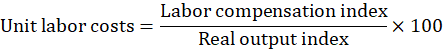
Unit labor costs are the payments for labor services used to produce each unit of output. Unit labor costs can be thought of as either the ratio of labor compensation to real output or as the ratio of hourly compensation to labor productivity. Unit labor costs are calculated as the ratio of an index of current dollar labor compensation to an index of real output, where real output is either the real value-added output or real sectoral output depending on the output concept used for the industry or sector.
Aggregate measures of capital input (or capital services) each year are calculated through multiple steps.
The productive capital stock is the set of capital assets used to produce output. It is represented by a sum for each asset in each industry, constructed from data on real investment by each industry into various productive asset categories (e.g. kinds of equipment), along with estimates of how much output those assets will produce, and how assets of various kinds decline in efficiency over time.
The capital stock is constructed using investment data by asset type and industry, the average service lives of assets, and assumptions about how assets deteriorate over time.
The productive capital stock is constructed using the perpetual inventory method, which sums all past capital asset investments, discounting older ones for deterioration, obsolescence, and eventual end-of-service-life. Each type of asset has an average service life inferred from survey data. The service life is the duration of the asset’s usefulness, until it is useless or withdrawn from service permanently. Service lives for each asset type are assumed to vary around that average, with an approximately normal distribution over a several-year period. Service lives vary because capital goods are made differently or used differently, and the variation in service lives means that a sudden change in investment has a slower and more diffuse effect on the capital stock. Overall, the model assumes that an increasing fraction of assets purchased at time t are withdrawn from service over time.
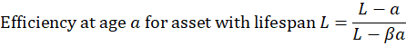
Within each service life, assets are assumed to decline in effectiveness at an increasing rate, according to a hyperbolic age-efficiency function. The age-efficiency function represents decline through deterioration and obsolescence, both of which can reduce productivity directly or require more downtime for repairs. All these avenues cause the age-efficiency function for an individual asset to be concave with respect to age. The decline is parameterized by the equation below, where a is age and L is service lifetime. Equipment is assumed to degrade earlier in its service life than structures do, with parameter  being .5 for equipment and .75 for structures. The efficiency computed is a fraction in the range of zero to one, which represents a proportion of the asset’s original effectiveness.
The productive capital stock for each asset-by-industry category is a sum of earlier investments in that asset, reduced according to the service life distribution and the age-efficiency function. Productive capital stocks of each asset in each industry are combined by Törnqvist aggregation to prepare productive stocks characterizing an entire industry, or a national total for the asset across industries.
The wealth stock is the value of existing stocks of capital assets, discounted to reflect the future services expected from them. The wealth stock is calculated as the sum of prior constant dollar capital investments after adjusting them for value loss due to aging and obsolescence of the assets. The wealth stock is calculated for each asset type as:

where the cohort age-price function for an asset is given as the integral of the product of the distribution of expected service lives for an asset with a particular age and the price of the asset at that expected service life.

The limits of the integral are the upper and lower bounds of the distribution of service lives, which are  and
and  respectively, where
  is the average service life of the asset type. The distribution of expected service lives is a modified truncated normal distribution with average and standard deviation
  . The normal distribution is truncated at ±2 standard deviations
  . This shifts the density function downward so that it equals zero at the upper and lower bounds of the distribution and then inflates the density function proportionately so that the final modified density integrates to 1. The price of the asset at the expected service life is indexed to 1 at the beginning of the vintage series.
The wealth stock depreciation rate is the rate at which the value of an asset or group of assets declines with age. It is calculated as a ratio where the numerator is real capital investment minus the change in the capital wealth stock from the previous period to the current period and the denominator is the average real value of the capital wealth stock over the current period and the previous period. However, the change in wealth stock can be volatile and for major industries, the productivity stock is used in the denominator.
For major industries:

For 4-digit industries:

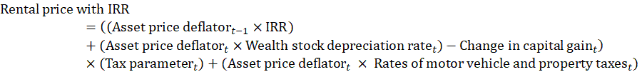
The rental price of capital,or the user cost of capital, is the opportunity cost of holding and using capital assets for a period of time. Users of capital typically own the capital used in production; therefore, prices and quantities of capital input are not observed. The equilibrium rental price is equal to the foregone earnings invested in the asset plus the decline in the asset’s value.
IRR is the internal rate of return. If the internal rate of return is negative or otherwise outside of acceptable values, the external rate of return (ERR) is used.


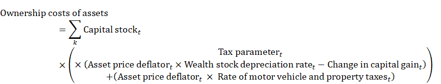
Ownership costs of assets per period are calculated as the productive capital stock times a tax parameter times a value given by the product of the capital deflator and wealth stock depreciation rate minus the change in capital gain plus the rate of asset state and local taxes. It is a sum over the k assets.
The internal rate of return (IRR) is the implied rate of return on investments in capital purchases that is calculated at the industry level. In other words, this rate is “internal” to each industry. BLS sets capital costs equal to the capital productive stock times the rental price. The equation is then reorganized to solve for the internal rate of return. This results in the internal rate of return being equal to capital costs minus the ownership costs of all assets, all divided by the stock value of all assets.
The IRR is given by the following calculation:

The external rate of return is a weighted average of calculated internal rates of return of private industries. This aggregate rate of return in the economy can be used for industries whose calculated internal rate of return is not economically plausible.
Capital costs are the payments to capital input used in the production of output. For the aggregated National Income and Product Account industries, capital costs are calculated as the sum of corporate capital payments and noncorporate capital payments.

For 4-digit NAICS manufacturing industries, capital costs are calculated as the residual after subtracting labor compensation and intermediate input costs from sectoral output.

The stock value of assets is the sum across all assets k of asset values given by the following:

The rental priceused is an approximation of the price to rent a unit of capital for a given period of time. The rental price calculation uses the industry’s internal rate of return or, when necessary, an economy-wide external rate of return.
Capital input is the contribution to production from capital assets. Capital input indexes for industries are calculated as the chained Törnqvist aggregate of productive capital stocks of the industry’s capital assets.

where the asset group cost share is defined as the average over two consecutive years:


Capital costs based on external rate of return (ERR) are calculated using a general rate of return across the entire private business sector. They are calculated as the sum of current dollar corporate capital and current dollar noncorporate capitalusing the external rate of return.

Capital costs based on internal rate of return are calculated using the rate of return to investment specific to the industry examined. They are calculated as the sum of current dollar corporate capital and current dollar noncorporate capital using the internal rate of return.

Capital costs used are the actual capital cost values used in productivity calculations after determining whether to base them on external or internal rates of return, which can vary by industry.
Nonlabor costs is a series that is specific to the nonfinancial corporate business sector. Nonlabor costs include consumption of fixed capital, taxes on production and imports less subsidies, net interest and miscellaneous payments, and business current transfer payments. Nonlabor costs are calculated as nonlabor payments minus profits, rental income of persons, and the current surplus of government enterprises.

Unit nonlabor costs are the nonlabor costs associated with each unit of output produced. Unit nonlabor costs are calculated as 100 times the ratio of an index of current dollar nonlabor costs to an index of real value-added output.

Nonlabor payments are output minus labor compensation. They include profits, consumption of fixed capital, taxes on production and imports less subsidies, net interest and miscellaneous payments, business current transfer payments, rental income of persons, and the current surplus of government enterprises. Nonlabor payments are calculated as combined inputs costs minus labor compensation.

Unit nonlabor payments are the nonlabor payments associated with each unit of output produced. Unit nonlabor payments are calculated as 100 times the ratio of an index of current dollar nonlabor payments to an index of real value-added output.

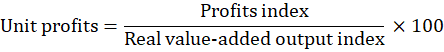
Unit profits are profits per unit of real value-added output, where profits are corporate profits before taxes with adjustments for inventory valuation and capital consumption. This measure is computed as 100 times the ratio of an index of profits divided by an index of real value-added output.
The contribution of capital intensity to labor productivity is the portion of labor productivity change attributed to the change in capital input relative to an index of hours worked.

The contribution of capital input excluding intellectual property products (IPP) and information processing equipment (IPE) intensity to labor productivity is the portion of labor productivity change attributed to the change in the capital input excluding intellectual property products and information processing equipment relative to an index of hours worked.

The contribution of IPE intensity to labor productivity is the portion of labor productivity change attributed to the change in information processing equipment capital input relative to an index of hours worked. Information processing equipment capital includes asset types such as computers and communications equipment.

The contribution of IPP excluding R&D intensity to labor productivity is the portion of labor productivity change attributed to the change in intellectual property products capital input excluding R&D relative to an index of hours worked. Intellectual property products capital consists of software, research and development (R&D), and artistic original assets.

The contribution of R&D intensity to labor productivity is the portion of labor productivity change attributed to the change in research and development input relative to an index of hours worked.

This section explains how to calculate input indexes for energy (E), materials (M), and services (S). For detailed manufacturing industries, quantity indexes of energy, materials, and services are calculated by dividing the input’s cost index by a price deflator: Quantity = Cost / Price.
An energy inputindex summarizes the fuels, electricity, and other forms of energy used to produce goods and services.
For major industries, energy input is the chain quantity index of energy from the U.S. Bureau of Economic Analysis GDP by Industry accounts. Energy costs are the payments to purchase energy for use in the production of output and also come from the GDP by Industry accounts. When appropriate, source values of energy are adjusted to a sectoral basis so that the value of production is equal to the value of combined inputs from the supplying industries.
For detailed manufacturing industries, energy input consists of electricity and fuels. Cost of electricity, quantity of electricity, and cost of fuels data are available from the U.S. Census Bureau. Price of fuels is estimated by aggregating BLS fuel producer price indexes (PPIs) and applying weights from the Energy Information Administration’s (EIA) Manufacturing Energy Consumption Survey (MECS). A real energy index is a combined Tornqvist aggregate of electricity and fuels indexes, using average shares of electricity and fuel costs as weights.

Materials input is the goods and commodities that are consumed, combined, and/or transformed in the production process to create other goods and services.
For major industries, materials input is the chain quantity index of materials from the Bureau of Economic Analysis GDP by Industry accounts. For goods-producing major industries, intrasectoral transactions are removed from the measure. Current dollar intrasectoral value is deflated using the industry gross output price deflator.


For detailed manufacturing industries, cost of materials data are available from the Census and are adjusted to remove intra-industry transfers. Materials price deflators are constructed for each industry by combining producer price indexes (PPIs) and import price indexes from BLS for detailed commodities. The deflators are combined using weights based on detailed commodity data from the Bureau of Economic Analysis (BEA) benchmark input-output tables and import matrices.
Indexes of real materials are calculated for each industry by dividing the materials costs index with the materials price deflator.

Services input is the services purchased from an outside entity, including contract work, for use in the production of output.
For major industries, services input is the chained quantity index of services from the Bureau of Economic Analysis GDP by Industry accounts. For service-providing major industries, intrasectoral transactions are removed from the measure. Current dollar intrasectoral value is deflated using the industry gross output price deflator.

For detailed manufacturing industries, services costs are estimated using multiple imputation methods. First, ratios of services to materials commodities are calculated from the BEA benchmark input-output use tables. The services-to-materials ratios are then interpolated between BEA benchmark years and applied to annual materials costs to derive an annual series of cost of services.

Data from the BEA KLEMS industry accounts are used to extend the services costs series before and after the BEA benchmark years.
Services price deflators are constructed for each industry by combining BLS consumer price indexes (CPIs), producer price indexes (PPIs), and deflators developed by the BEA. The deflators are combined using weights based on detailed commodity data from the BEA benchmark input-output tables.

Intermediate inputs are the purchased energy, materials, and services (E, M, and S) used to produce industry output. BLS excludes purchases made from establishments within the producing industry.
For major industries, energy, materials, and services inputs are based on the BEA annual input-output tables. Törnqvist indexes of each of these three types of input are prepared at roughly the three-digit NAICS level. Materials and services inputs are adjusted to exclude transactions between establishments within the same industry or sector.
For detailed manufacturing industries, the value of material inputs is calculated by dividing an industry’s current-dollar materials purchases by a price deflator. Materials price deflators are constructed for each industry by combining producer price indexes and import price indexes for the commodities used by that industry, with weights based on detailed commodity data from the BEA input-output tables. Price indexes for business services are constructed similarly, using CPIs, PPIs, or BEA deflators. The value of fuels used by each industry is deflated similarly, based on PPIs for various fuel categories, weighted by the industry’s fuel expenditures from the Energy Information Administration (EIA).
The separate indexes of real materials, services, fuels, and energy are combined into a total intermediate inputs Törnqvist index. The weights for each component reflect each input’s share of the cost of intermediate inputs, averaged between consecutive years. This index can be computed equivalently from the energy, materials, and services indexes above, or from the arrays of underlying quantities and prices of these inputs.

Combined inputs are the aggregate of measured inputs that are used to produce output. These include capital, labor, energy, materials, and services. For sectoral production, the combined inputs are adjusted to avoid double counting among the intermediate inputs (energy, materials, and services) during industry aggregation. At each level of industry aggregation, shipments of intermediate inputs among establishments are removed. In this way, the combined inputs measure only includes the combined inputs that were used in the production of final goods that left the industry at each level of aggregation.
Combined inputs for value-added production is calculated as the cost-share-weighted Törnqvist index of capital input and labor.

For sectoral production output concepts, the combined inputs are calculated as the cost-share-weighted Törnqvist index of capital input, labor input, and the combined intermediate inputs.

Finally, for sectoral output concepts with detailed intermediate inputs, combined inputs is calculated as the cost-share-weighted Törnqvist index of capital input, labor input, energy input, materials input, and services input.

Combined inputs costs are the payments and implicit compensation to utilize all inputs to produce output.Combined inputs costs for value-added production are calculated as the sum of current dollar capital costs and current dollar labor compensation.

Combined inputs costs are equal to value-added production in this framework.
Combined inputs costs for sectoral production with combined intermediate inputs are calculated as the sum of current dollar capital costs, current dollar labor compensation, and current dollar combined intermediate inputs.

Combined inputs costs for sectoral production with detailed intermediate inputs are calculated as the sum of current dollar capital costs, current dollar labor compensation, and current dollar detailed intermediate inputs.

Combined inputs costs are equal to sectoral output in these two combined inputs costs concepts. The combined inputs costs index for these concepts is calculated as 100 times the current dollar combined inputs costs in a given year divided by the current dollar combined inputs costs in the base year b.

Unit combined inputs costs are the total costs incurred for each unit of output produced. They are calculated as the current dollar combined inputs index divided by an index of real output, where output can be either value-added or sectoral, multiplied by 100.

The contribution of energy intensity to labor productivity is the portion of labor productivity change attributed to the change in energy input relative to an index of hours worked.

The contribution of materials intensity to labor productivity is the portion of labor productivity change attributed to the change in materials input relative to an index of hours worked.

The contribution of services intensity to labor productivity is the portion of labor productivity change attributed to the change in services input relative to an index of hours worked.

The contribution of intermediate inputs intensity to labor productivity is the portion of labor productivity change attributed to the change in intermediate inputs relative to an index of hours worked.

This section explains how to calculate measures tied specifically to prices.
The consumer price deflator is an index that measures changes in the level of consumer prices. The Consumer Price Index is not calculated or produced by OPT. It is obtained from the BLS Office of Prices and Living Conditions (OPLC). However, the consumer price deflator used to compute quarterly and annual measures of real hourly compensation by major sector is constructed by OPT using two measures published by OPLC. Changes for recent quarters are based on quarterly averages of the monthly Consumer Price Index for all urban consumers (CPI-U). Changes are based on quarterly averages of the monthly Consumer Price Index Retroactive series (CPI-U-RS) from first-quarter 1978 through the last complete calendar year for which it is has been published.
The sectoral output price deflator is the relative change in the price of sectoral output over time. The sectoral output price deflator is calculated as 100 times a current dollar sectoral output index divided by real sectoral output.

The value-added output price deflator is the relative change in the price of value-added output. When using a value-added output concept, the value-added price deflator is calculated as 100 times a current dollar value-added output index divided by real value-added output.

The labor price deflator is the relative change over time in the payments to labor for the production of output. The labor price deflator is calculated as 100 times a current dollar labor compensation index divided by an hours worked index.

For each type of asset, its capital asset price deflator is the relative change over time in the cost to acquire it. A capital asset price deflator is calculated as 100 times the ratio of the sum of current dollar investment in an asset across industries (Ind) to the sum of constant dollar investment in the asset.

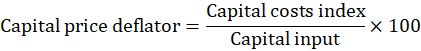
The capital price deflator is the relative change over time in the cost to utilize units of capital input to produce output. The capital price deflator is calculated as 100 times a current dollar capital costs index divided by real capital input.
Capital rental prices are the prices paid to rent various kinds of capital assets used in the production of output.
Such assets are typically owned by producing firms, rather than rented, so capital rental prices are typically not observable in explicit transactions. Consequently, rental prices are usually implicit, and are estimated rather than observed.
The rental price is equal to the foregone earnings invested in the asset plus the decline in the asset’s value. In its simplest form, the rental price for a period is set to the price of the asset multiplied by the sum of the rate of depreciation and the appropriate rate of return. BLS also accounts for the effects of inflation on the price of new assets and of taxes. The capital rental price for an asset is calculated as the product of a tax term and an asset price term divided by 1 minus the corporate income tax rate. This value is then added to the product of the asset price from the previous period and the current rate of asset state and local taxes.

The tax term is calculated as 1 minus the corporate income tax rate minus the present value of $1 of the depreciation deduction.

The asset price term is the product of the asset price (P) from the previous period and the industry-specific rate of return on capital plus the product of the asset price from the previous period and the average rate of economic depreciation of the asset in a particular industry minus the change in the 3-year moving average of the asset price.

The rate of asset state and local taxes is calculated as the industry motor vehicle or property tax value divided by the sum of industry motor-vehicle- or property-tax-related asset capital stock.
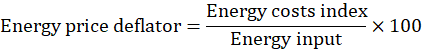
The energy price deflator is the relative change over time in the cost to acquire units of energy to produce output. The deflator is an index that is calculated as 100 times the current dollar energy costs index divided by energy input.
The materials price deflator is the relative change over time in the cost to acquire units of materials to produce output. The deflator is an index that is calculated as 100 times the current dollar materials costs index divided by materials input.

The services price deflator is the relative change over time in the cost to acquire services input to produce output. The deflator is an index that is calculated as 100 times the current dollar services costs index divided by services input.

The intermediate inputs price deflator is the relative change over time in the cost to acquire intermediate inputs to produce output. The deflator is an index that is calculated as 100 times the current dollar intermediate inputs costs index divided by intermediate inputs.

The combined inputs price deflator is the relative change over time in the value of money spent to use all inputs for production. This information helps make combined input utilization in different time periods comparable. The deflator is an index that is calculated as 100 times the current dollar combined inputs costs index divided by combined inputs.

Seasonal fluctuations in economic time series can make it difficult to see underlying trends and changes. Seasonal factors can also obscure business cycle patterns in the time series. Therefore, it is necessary to remove the seasonal effects from both output and hours worked for productivity measurement. Seasonal adjustment attempts to decompose movements in time series into a few components, one of which is seasonality, and then remove the seasonality. For quarterly labor productivity measurement, we need seasonally adjusted series of real output and hours worked. The real output measures used to compute quarterly measures of labor productivity for the U.S. business and nonfarm business sectors are seasonally adjusted and published by the BEA. Thus, the task for BLS is seasonal adjustment of measures of hours worked.
Hours worked for quarterly labor productivity measures rely primarily upon data from the BLS CES program, which provides seasonally adjusted data on employees in nonfarm establishments. To supplement these data, OPT uses data from the CPS to construct estimates of employment and hours at work for proprietors and partners (the unincorporated self-employed) and unpaid family workers in the farm and nonfarm sectors. CPS data on employment and hours of postal workers and public administration workers are used to calculate average weekly hours of federal, state, and local government enterprises employees. These series are combined with employment from BEA and CES to calculate hours for workers in government enterprises, the last component needed to calculate business sector hours. OPT compiles the not seasonally adjusted CPS data and then seasonally adjusts the series.
OPT seasonally adjusts any monthly and quarterly CPS series that underlie the quarterly measures of hours worked using X-13ARIMA-SEATS, a software package developed by the U.S. Census Bureau and enhanced by Statistics Canada and the Bank of Spain. Each year, the series are reevaluated to determine the parameters to use for the coming year. The data are also revised back 5 years for the March release, which necessitates the recalculation of seasonal factors over that time frame.
This section focuses on intermediate capital calculations, including property tax, motor vehicle tax, and the tax parameter.
Property tax is the tax rate for property used to determine the rental price of property-related assets. The property tax is calculated as the total property tax divided by the sum of productive stocks of structures, residential structures, and land.

Motor vehicle tax is the tax rate for autos, trucks, buses, and trailers used to determine the rental price of motor-vehicle-related assets. The motor vehicle tax is calculated as total motor vehicle tax divided by the vehicle productive stock.

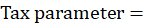
The tax parameter is the combination of the corporate income tax, the present value of $1 of tax depreciation allowances, and the effective rate of investment tax credit used to determine the implicit rental price of capital assets. The tax parameter is calculated as a numerator of 1 minus the product of the maximum corporate income tax rate and the present value of $1 of tax depreciation allowance minus the effective investment tax credit rate, all divided by 1 minus the maximum corporate income tax rate.

The present value of $1 tax depreciation allowance is calculated based on the Moody’s AAA bond rate, the asset service life for tax purposes, and the depreciation function.
This section explains how to calculate supplemental productivity measures, including capital productivity, energy productivity, materials productivity, services productivity, intermediate inputs productivity, and output per worker.
Capital productivity is the efficiency at which capital input is used to produce output. BLS calculates capital productivity for industries and major sectors as part of the TFP measures. Capital productivity is the ratio of real output to capital input.
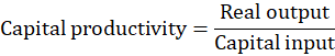
Output can be defined using either the value-added (for major sectors) or sectoral output (for industries) concept.
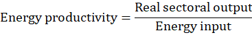
Energy productivity is the efficiency at which energy inputs are used to produce output. BLS calculates energy productivity for industries as part of the KLEMS TFP measures. Energy productivity is the ratio of real sectoral output to energy inputs.
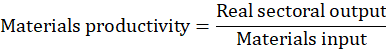
Materials productivity is the efficiency at which material inputs are used to produce output. BLS calculates materials productivity for industries as part of the KLEMS TFP measures. Materials productivity is the ratio of real sectoral output to materials inputs.
Services productivity is the efficiency at which services inputs are used to produce output. BLS calculates services productivity for industries as part of the KLEMS TFP measures. Services productivity is the ratio of real sectoral output to services inputs.

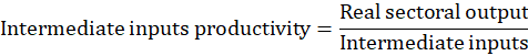
Intermediate inputs productivity is the efficiency at which intermediate inputs are used in the production of output. Intermediate inputs productivity is the ratio of real sectoral output to intermediate inputs.
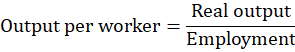
Output per worker is the efficiency at which output is produced by workers. Output per worker is the ratio of real output to employment. Real output can be either real value-added or real sectoral output.
This section explains how to calculate supplemental labor measures, including labor compensation, hourly compensation, real hourly compensation, and labor share.
Labor compensation is the total of payments to labor to produce output, including wages, benefits, and other monetary or nonmonetary payments. The main portion of labor compensation is employee compensation, which is a comprehensive measure that includes wages and salaries; commissions; tips; bonuses; severance payments and early retirement buyout payments; regular supplementary allowances; exercising of nonqualified stock options; payments in kind, such as transit subsidies, meals, and lodging; and employer contributions to private and government pension funds and social insurance. BEA provides compensation of employees on a national basis, which is adjusted to match the business sector definition. The measure of compensation also includes all workers rather than all employees, which means compensation for the unincorporated self-employed (proprietors and partners) is included. Labor compensation for unincorporated self-employed workers is calculated using different methods depending on the available data.

Hourly compensation is the sum of wages and benefits paid per hour of work. Hourly compensation is calculated as the ratio of labor compensation to hours worked.

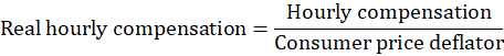
Real hourly compensation is the average wages and benefits paid per hour, adjusted for inflation. Real hourly compensation is calculated as the ratio of current dollar hourly compensation to the consumer price deflator (defined above).
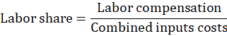
Labor share is the proportion of current-dollar output that accrues to workers in exchange for their labor. When using value-added production, labor share is calculated as the ratio of labor compensation to value-added output.
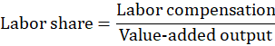
When sectoral production is the output concept, labor share is calculated as the ratio of labor compensation to combined inputs costs.
This section explains how to calculate supplemental capital measures, including capital composition, capital input to wealth stock ratio, capital intensity, capital share, productive capital stock to wealth stock ratio, and unit capital costs.
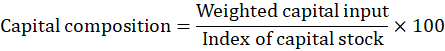
Capital composition is the portion of change in capital input that cannot be attributed to changes in capital stock. Capital composition is calculated as 100 times the weighted capital input divided by the index of constant dollar productive capital stock.
Thecapital input to wealth stock ratio is the ratio of capital input to the value of existing stocks of capital assets, discounted to reflect the future services expected from them. The capital input to wealth stock ratio is calculated as 100 times the ratio of capital input to the index of wealth stock.

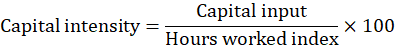
Capital intensityis the ratio of the amount of capital input used relative to the amount of labor hours used to produce output. Capital intensity is calculated as 100 times the ratio of capital input to an index of hours worked.
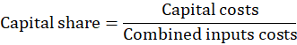
Capital share is the proportion of current-dollar output production attributed to the use of capital input. Capital share is calculated as the current dollar capital costs divided by combined inputs costs.
Theproductive capital stock to wealth stock ratio is the ratio of the implicit amount of new investment that would be required to produce the same present-day services as the existing level of capital assets to the value of existing stocks of capital assets, discounted to reflect the future services expected from them. The productive capital stock to wealth ratio is calculated as the index of productive capital stock divided by the index of the wealth stock.

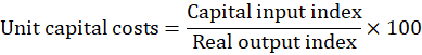
Unit capital costs are the payments for capital input used to produce each unit of output. Unit capital costs are calculated as 100 times an index of capital input divided by an index real output, where output can be either real value-added output or real sectoral output.
This section explains how to calculate measures of intensity.
Intermediate inputs intensity is the ratio of intermediate inputs to an index of hours worked.

Energy intensity in each period is the ratio of energy input to an index of hours worked.

Materials intensity is the ratio of materials input to an index of hours worked.