
An official website of the United States government
An official website of the United States government
The .gov means it's official.
Federal government websites often end in .gov or .mil. Before sharing sensitive information,
make sure you're on a federal government site.
The site is secure.
The
https:// ensures that you are connecting to the official website and that any
information you provide is encrypted and transmitted securely.
To assist users in ascertaining the reliability of Employment Cost Index (ECI) series, standard errors of all estimates, excluding seasonally adjusted and constant dollar series, are made available with each publication. Standard errors provide a measure of the precision of an estimate to ensure that it is within an acceptable range for its intended purpose. These standard errors are available through the public database and in spreadsheet format.
The ECI is derived from a sample survey and thus, it is subject to sampling errors. Standard errors relate to differences that occur from sampling errors, but not from nonsampling errors.
Sampling errors are differences between the results computed from a sample of observations and those computed from all observations in the population. In the case of the ECI, the population of an estimate is an industry or occupation in the civilian, private, or state and local government sector. Estimates derived from different samples selected using the same sample design may differ from each other.
Nonsampling errors are not measured. One type of nonsampling error is survey nonresponse, when survey respondents are unwilling or unable to participate in the survey. Other nonsampling errors include inaccurate or incorrectly entered data, and processing errors. BLS quality assurance programs contain procedures for reducing nonsampling errors. These procedures include data collection reinterviews, observed interviews, and systematic reviews of collected data. Finally, field economists (data collectors) undergo extensive training to maintain high data collection standards.
Standard errors can be used to measure the precision with which an estimate from a particular sample approximates the expected result (value) of all possible samples (population). The chances are about 68 out of 100 that an estimate from the survey differs from a population result within one standard error.
Standard errors can be used to calculate confidence intervals around an estimate. With a 90 percent confidence interval, the chances are about 90 out of 100 that this difference would be within 1.645 standard errors. If all possible samples were selected and an estimate of a value and its sampling error were computed for each, then (for approximately 90 percent of the samples) the intervals from 1.645 standard errors below the estimate to 1.645 standard errors above the estimate would include the "true" average value.
Evaluate the statement: “From March 2025 to June 2025, total compensation for private industry workers, not seasonally adjusted, increased 1.1 percent with a standard error of 0.09.”
Confidence interval = estimate +/- (standard error * critical value)
90% confidence interval = estimate +/- (standard error * 1.645)
= 1.1 +/- (0.09 * 1.645)
= 1.1 +/- 0.1481
≈ [1.0, 1.2]
If all possible samples were drawn from the target population, and each time a new estimate and confidence interval were calculated, then 90 percent of those confidence intervals would contain the true population value. Therefore, we are 90 percent confident that the interval [1.0%, 1.2%] will contain all possible sample means with NCS sample design.
If you wish to calculate a 95 percent confidence interval, replace the critical value of 1.645 with 1.960. For a 99 percent confidence interval, use 2.576 as the critical value.
Comparative statements appearing in ECI publications are statistically significant at the 90 percent level of confidence, unless otherwise indicated. A statistically significant difference is a result that is not attributed to chance alone. Differences between estimates which may appear to be substantial at first glance may not be statistically significant.
Evaluate the statement: “From June 2024 to June 2025, wages and salaries increased more for private industry workers in the Philadelphia-Reading-Camden, PA-NJ-DE-MD CSA (3.9 percent) than in the Boston-Worcester-Providence, MA-RI-NH CSA (2.8 percent).”
Step 1. Calculate a statistical significance test statistic
Philadelphia-Reading-Camden, PA-NJ-DE-MD CSA: 3.9 percent change with 0.40 standard error
Boston-Worcester-Providence, MA-RI-NH CSA: 2.8 percent change with 1.43 standard error
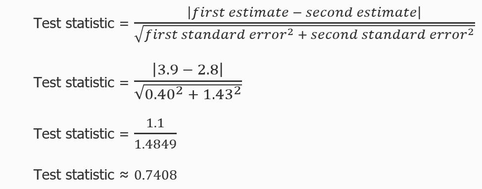
Step 2. Compare against the critical value
A difference is statistically significant if the test statistic is greater than the critical value.
0.7408 < 1.645
The test statistic (0.7408) is less than the critical value (1.645). Therefore, the difference between the estimates is not statistically significant. That is, the comparative statement that wages and salaries increased more for workers in the Philadelphia-Reading-Camden, PA-NJ-DE-MD CSA than for workers in the Boston-Worcester-Providence, MA-RI-NH CSA does not pass the statistical significance test.
Note: examples are for illustrative purposes only and are not intended to represent current data.
For a more detailed explanation of standard errors, including how they are calculated, see the section Calculating estimate reliability in the Handbook of Methods: Calculation.
Last Modified Date: September 30, 2025