
An official website of the United States government
An official website of the United States government
The .gov means it's official.
Federal government websites often end in .gov or .mil. Before sharing sensitive information,
make sure you're on a federal government site.
The site is secure.
The
https:// ensures that you are connecting to the official website and that any
information you provide is encrypted and transmitted securely.

Crossref 0
Economic precariousness: A new channel in the housing market cycle, International Journal of Finance & Economics, 2019.
Returning to the Nest: Debt and Parental Co-Residence Among Young Adults, Finance and Economics Discussion Series, 2014.
Heterogeneity in House Price Dynamics, SSRN Electronic Journal , 2017.
Regional US House Price Formation: One Model Fits All?, SSRN Electronic Journal, 2014.
Geographically Weighted Regression Models in Estimating Median Home Prices in Towns of Massachusetts Based on an Urban Sustainability Framework, Sustainability, 2018.
Central American immigrant mothers' narratives of intersecting oppressions: A resistant knowledge project, Journal of Marriage and Family, 2022.
Returning to the Nest: Debt and Parental Co-Residence Among Young Adults, SSRN Electronic Journal, 2014.
Residential mobility during adolescence: Do even “upward” moves predict dropout risk?, Social Science Research, 2015.
Defending Gentrification as a Valid Collective Conception: Utilizing the Metanarrative of “Suburbia” as a Common Axis for the Diversity of Middle-Class Reurbanization Projects, Urban Affairs Review, 2019.
It is now well established that the U.S. housing market crisis preceded the labor market crisis and that, in the wake of these crises, doubling up and cohabitation increased and homeownership fell. What is less clear, however, is what happened at the subnational level. This article reports on (1) how the length, severity, and relative timing of both the housing and labor market crises varied by metropolitan statistical area (MSA), and (2) the association between the timing of these crises and changes in homeownership and doubling up at the MSA level. The analysis uses data on 353 MSAs, with a focus on 12 MSAs, for the period from 2005 (precrisis) to 2011. MSAs are categorized into those where the housing market declined first, those where the labor market declined first, and those where the events were concurrent. The analysis reveals that (1) in the majority of MSAs, the labor market declined first, contrary to the national pattern and the experience of the vast majority of large MSAs; (2) there is a clear relationship between greater regional housing distress and falling homeownership rates; and (3) somewhat surprisingly, the association between changes in doubling up and these crises is fairly weak at the MSA level.
In early 2007, the most recent U.S. housing bubble burst. The bust was followed by the onset of the Great Recession and the deepest employment decline that the United States has experienced since the end of World War II.1 In the wake of these events, media reports and research studies have documented increased “doubling up” of families as well as increased numbers of young adults who returned to their parents’ homes or were slower to exit them than they were in years past.2, 3 A sign of the times, a 2009 USA Today article began, “Love isn’t all that’s keeping family together today. The bruising housing market is too.”4 Other reports have pointed to rising rates of cohabitation resulting from the economic crisis, in addition to the secular rise that was already underway.5
Although these national patterns are now well established, the relative timing of the housing and labor market crises at the MSA level and the association of these crises with household formation have not been fully studied.6 This article reports on (1) how the length, severity, and relative timing of both the housing and labor market crises varied by MSA, and (2) the association between the timing of these crises and changes in homeownership and doubling up at the MSA level. The analysis uses data on 353 MSAs, with a focus on 12 MSAs, for the period from 2005 (precrisis) to 2011.
In this article, MSA-level housing prices serve as a measure of overall housing conditions. The start of the housing crisis in a given area is identified by looking at when housing prices peaked. Similarly, the start of the labor market crisis in a given area is identified by looking at when employment peaked. Using information on the timing of each crisis, the article then looks at the relative timing of the crises for each of the 353 MSAs examined, by investigating (1) whether the housing market crisis occurred first (which was the pattern observed for the nation as a whole), (2) whether the labor market crisis occurred first (which, it turns out, was the pattern for a slight majority of MSAs), and (3) whether these events were concurrent. The relative timing of the crises appears to be a useful way to categorize MSAs. The MSAs where the housing market declined first have some distinct characteristics: many are among the largest MSAs (as measured by employment size), and the crises in these MSAs were among the most severe, in terms of both magnitude and duration.
The article also investigates the association between the housing and labor market crises and changes in doubling up and homeownership at the MSA level. As would be expected, there is a strong association between greater regional housing distress and falling homeownership rates. Somewhat surprisingly, however, the association between changes in doubling up and these crises appears fairly weak at the MSA level.
The collapse of the U.S. housing market in 2007 and the onset of the Great Recession spawned a tremendous amount of inquiry into the nature, causes, and consequences of these crises. The most relevant previous research can be divided into two parts: (1) studies that have looked at the housing market crisis or the labor market crisis at the subnational level, and (2) studies that have looked at the relationship between these crises and household formation at the MSA level. Each literature is discussed in turn.
A number of studies have examined the recent boom and subsequent bust in the national housing market. Estimates of the housing boom’s start date vary, with suggested possibilities including 1996, 1998, and 2002.7 There is a much narrower band around the date when the national housing bubble burst; the bust occurred in either mid-2006 (estimated using the Case–Shiller Home Price Indices) or in first quarter 2007 (estimated using the House Price Index from the Federal Housing Finance Agency [FHFA]).8 Turning to subnational data, some studies point to considerable dispersion across MSAs in the magnitude of the rise in prices during the boom as well as in the decline of prices during the bust.9 These studies also find a similar set of patterns: (1) MSAs located in the interior of the United States (e.g., Charlotte, Detroit, Cleveland, and Chicago) experienced smaller increases in housing prices during the boom than did MSAs located on the coasts; and (2) the set of MSAs that experienced larger booms also tended to be those which experienced larger busts. Among the interesting exceptions is Las Vegas. In Las Vegas, the rise in nominal housing prices during the boom (150 percent) was not quite as large as that for some other West Coast cities (in both Los Angeles and San Diego housing prices increased more than 200 percent), and the decline in housing prices during the bust was considerably larger than the decline for these counterparts (62 percent in Las Vegas versus around 40 percent in both Los Angeles and San Diego).10
Some studies have also looked at the subnational variation in the timing of housing booms and busts.11 A study by Todd Sinai is the most relevant here, because it looked at both the timing of the most recent housing boom and the timing of the housing bust, and drew comparisons with the housing cycle of the 1980s.12 Interestingly, the study found that the timing in MSAs of the most recent housing bust was more closely concentrated than that of the previous bust, with many peaks around 2007 and 2008 but still a good deal of heterogeneity. Unlike the present article, however, the study did not look at more finely grained (quarterly) data or consider variations in the timing of events in the labor market relative to the housing market by MSA.
Extensive evidence also points to substantial heterogeneity in employment conditions at the subnational level during the latter part of the 2000s. MSAs that were especially hard hit by the labor market crisis, as measured by Bureau of Labor Statistics (BLS) local area unemployment rates, include Detroit, Las Vegas, Los Angeles, and Miami. With the notable exception of Detroit from this set, these MSAs also experienced the housing bubble.13 This is to be expected given the strong relationship between the health of the housing sector and the level of construction employment.14 Although less attention has been paid to regional variations in the timing of employment crises, Howard Wall conducted one such study.15 Wall examined the timing of economic expansions and employment downturns for a small number of cities. He found that these cities experienced these events at around the same time the nation did; however, in line with Sinai’s conclusion regarding variation in the timing of housing crises at the MSA level, Wall still identified quite a bit of dispersion.
In addition, a few previous studies have sought to explicitly link changes in the housing market and/or the labor market during the recent crisis to changes in household formation at the MSA level.16 For example, Timothy Dunne used MSA-level data on people ages 18 to 34 to investigate the correlation between household formation (e.g., headship rates17 and number of households) and labor market conditions and the correlation between household formation and housing prices.18 Although he found that doubling up is associated to some extent with both a weak housing market and a weak labor market, he did not probe further. Gary Painter also used data on 80 MSAs from the American Community Survey (ACS) for the period 2005–2008 to examine changes in household headship, homeownership, and overcrowding within a dwelling for MSAs grouped by immigrant status.19 His study found that headship rates and overcrowding rose while homeownership declined for all groups examined, although to differing extents.
Finally, it is worthwhile pointing to a few studies that have used MSA-level data to investigate associations between the housing crisis and other outcomes. Lisa Dettling and Melissa Kearney, for instance, used MSA-level data to examine the relationship between variations in housing prices and fertility during the recent crisis.20 In addition, a number of studies have looked at spillover and contagion effects of the foreclosure crisis that accompanied the burst of the housing bubble.21
To sum up, this article builds upon earlier studies of subnational housing and labor markets and documents geographic differences in the timing and severity of the housing and labor market crises of the late 2000s. It then takes a further step and examines associations between these crises and household formation.
The analysis uses data on 353 MSAs, with a focus on 12 MSAs, for the period from 2005 to 2010 (and, where data were available, to 2011).22 The rationale for the selection of these specific MSAs is discussed shortly. Table 1 summarizes the key indicators for household formation and housing and labor market conditions, along with their data sources. Labor market conditions are principally measured using BLS data on nonfarm payroll employment.23 Overall conditions in the housing market are measured using the FHFA House Price Index for single-family units.24 In the analysis, the index is set to 100, with 2005 as the base year. These data are available at the quarterly level through 2011. Previous studies examining changes in overall housing conditions across MSAs have similarly used these data or relied on a smaller set of MSAs included in the Case–Shiller indices.25
| Variable | Definition | Source |
|---|---|---|
| Household formation and homeownership | ||
| Household size | Size of household | ACS |
| Nonrelatives in family households (percent) | Nonrelatives living in family households as a percentage of total people in family households | ACS |
| Unmarried households (percent) | Unmarried (opposite-sex) partner households as a percentage of total households | ACS |
| Homeownership rate (percent) | Owner-occupied households as a percentage of total households | ACS |
| Housing market conditions | ||
| House Price Index (2005 = 100) | Prices for single-family-unit transactions serviced by Fannie Mae or Freddie Mac | FHFA |
| Foreclosure rate (percent) | (number of foreclosures / number of loans) x 100; measure is akin to a default rate | CoreLogic |
| Labor market conditions | ||
| Employment (thousands) | Nonfarm payroll employment, age 16 and over | BLS |
| Unemployment rate | Rate calculated for civilian noninstitutional population, age 16 and over | BLS |
Some attention is also focused on foreclosures, given the acute impact they had on particular housing submarkets (e.g., subprime lending). Foreclosures are measured using proprietary data obtained from CoreLogic, which includes 85 percent of foreclosures and first lien loans.26 CoreLogic defines a foreclosure as a situation in which an owner’s right to a property is terminated, usually because of default. The foreclosure rate is calculated here as foreclosures per number of loans (multiplied by 100). Foreclosure data are available at the monthly level, although in many of the analyses they are aggregated to the quarterly (or annual) level for comparisons with data from other sources. For all nonannual data, seasonal adjustment is undertaken using a locally weighted regression.27
Data on rates of doubling up, cohabitation, and housing tenure (home ownership) are drawn from ACS annual data for the period 2005–2010. The prime advantage of the ACS is that, as the largest household survey in the United States, it has information on 3 million addresses. In all analyses, group quarters (i.e., dorms and institutional settings) are omitted as a household type. Using the ACS, two measures of doubling up are examined: (1) average household size and (2) the number of nonrelatives living in family households as a percentage of total number of people residing in family households.28 For completeness, the article also examines homeownership rates, defined as the percentage of households that are owner occupied. In interpreting these measures, homeownership rates reflect the investment component of housing demand whereas rates of doubling up provide information regarding consumption demand for housing (e.g., need for shelter). Finally, the article also looks at trends in the number of unmarried (opposite-sex) partner households as a percentage of total households. This latter measure differs from doubling up in that it provides information about the marriage versus cohabitation decision. Although cohabitation rates have been experiencing a secular increase, economic conditions also play an important role, given evidence that couples are more likely to defer marriage until they are able to afford it.29
The empirical analysis proceeds in two parts. First, the severity and relative timing of the housing and labor market crises are examined for the 353 MSAs for which complete data are available. This analysis uses quarterly data from second quarter 2005 through fourth quarter 2011.30 This analysis further focuses on the experience of 12 MSAs with distinct differences in the relative timing of their housing and labor market crises. The second part of the analysis investigates the association between the housing and labor market crises and changes in homeownership and doubling up. In this second portion of the analysis, the quarterly data on the housing and labor market variables are annualized to match the annual data available in the ACS.
| Date | Variable | Value | Housing crisis | Recession and housing crisis | Postrecession and housing crisis |
|---|---|---|---|---|---|
January 2005 | Employment (millions, monthly) | 132.502 | 0 | 0 | 0 |
February 2005 | Employment (millions, monthly) | 132.742 | 0 | 0 | 0 |
March 2005 | Employment (millions, monthly) | 132.877 | 0 | 0 | 0 |
April 2005 | Employment (millions, monthly) | 133.239 | 0 | 0 | 0 |
May 2005 | Employment (millions, monthly) | 133.407 | 0 | 0 | 0 |
June 2005 | Employment (millions, monthly) | 133.653 | 0 | 0 | 0 |
July 2005 | Employment (millions, monthly) | 134.025 | 0 | 0 | 0 |
August 2005 | Employment (millions, monthly) | 134.217 | 0 | 0 | 0 |
September 2005 | Employment (millions, monthly) | 134.282 | 0 | 0 | 0 |
October 2005 | Employment (millions, monthly) | 134.363 | 0 | 0 | 0 |
November 2005 | Employment (millions, monthly) | 134.698 | 0 | 0 | 0 |
December 2005 | Employment (millions, monthly) | 134.856 | 0 | 0 | 0 |
January 2006 | Employment (millions, monthly) | 135.130 | 0 | 0 | 0 |
February 2006 | Employment (millions, monthly) | 135.446 | 0 | 0 | 0 |
March 2006 | Employment (millions, monthly) | 135.726 | 0 | 0 | 0 |
April 2006 | Employment (millions, monthly) | 135.907 | 0 | 0 | 0 |
May 2006 | Employment (millions, monthly) | 135.928 | 0 | 0 | 0 |
June 2006 | Employment (millions, monthly) | 136.008 | 0 | 0 | 0 |
July 2006 | Employment (millions, monthly) | 136.218 | 0 | 0 | 0 |
August 2006 | Employment (millions, monthly) | 136.397 | 0 | 0 | 0 |
September 2006 | Employment (millions, monthly) | 136.556 | 0 | 0 | 0 |
October 2006 | Employment (millions, monthly) | 136.553 | 0 | 0 | 0 |
November 2006 | Employment (millions, monthly) | 136.758 | 0 | 0 | 0 |
December 2006 | Employment (millions, monthly) | 136.927 | 0 | 0 | 0 |
January 2007 | Employment (millions, monthly) | 137.161 | 1 | 0 | 0 |
February 2007 | Employment (millions, monthly) | 137.251 | 1 | 0 | 0 |
March 2007 | Employment (millions, monthly) | 137.437 | 1 | 0 | 0 |
April 2007 | Employment (millions, monthly) | 137.513 | 1 | 0 | 0 |
May 2007 | Employment (millions, monthly) | 137.654 | 1 | 0 | 0 |
June 2007 | Employment (millions, monthly) | 137.734 | 1 | 0 | 0 |
July 2007 | Employment (millions, monthly) | 137.699 | 1 | 0 | 0 |
August 2007 | Employment (millions, monthly) | 137.675 | 1 | 0 | 0 |
September 2007 | Employment (millions, monthly) | 137.752 | 1 | 0 | 0 |
October 2007 | Employment (millions, monthly) | 137.838 | 1 | 0 | 0 |
November 2007 | Employment (millions, monthly) | 137.949 | 1 | 0 | 0 |
December 2007 | Employment (millions, monthly) | 138.042 | 0 | 1 | 0 |
January 2008 | Employment (millions, monthly) | 138.056 | 0 | 1 | 0 |
February 2008 | Employment (millions, monthly) | 137.971 | 0 | 1 | 0 |
March 2008 | Employment (millions, monthly) | 137.892 | 0 | 1 | 0 |
April 2008 | Employment (millions, monthly) | 137.677 | 0 | 1 | 0 |
May 2008 | Employment (millions, monthly) | 137.491 | 0 | 1 | 0 |
June 2008 | Employment (millions, monthly) | 137.322 | 0 | 1 | 0 |
July 2008 | Employment (millions, monthly) | 137.106 | 0 | 1 | 0 |
August 2008 | Employment (millions, monthly) | 136.836 | 0 | 1 | 0 |
September 2008 | Employment (millions, monthly) | 136.377 | 0 | 1 | 0 |
October 2008 | Employment (millions, monthly) | 135.905 | 0 | 1 | 0 |
November 2008 | Employment (millions, monthly) | 135.130 | 0 | 1 | 0 |
December 2008 | Employment (millions, monthly) | 134.425 | 0 | 1 | 0 |
January 2009 | Employment (millions, monthly) | 133.631 | 0 | 1 | 0 |
February 2009 | Employment (millions, monthly) | 132.936 | 0 | 1 | 0 |
March 2009 | Employment (millions, monthly) | 132.106 | 0 | 1 | 0 |
April 2009 | Employment (millions, monthly) | 131.402 | 0 | 1 | 0 |
May 2009 | Employment (millions, monthly) | 131.050 | 0 | 1 | 0 |
June 2009 | Employment (millions, monthly) | 130.578 | 0 | 0 | 1 |
July 2009 | Employment (millions, monthly) | 130.227 | 0 | 0 | 1 |
August 2009 | Employment (millions, monthly) | 130.017 | 0 | 0 | 1 |
September 2009 | Employment (millions, monthly) | 129.784 | 0 | 0 | 1 |
October 2009 | Employment (millions, monthly) | 129.614 | 0 | 0 | 1 |
November 2009 | Employment (millions, monthly) | 129.593 | 0 | 0 | 1 |
December 2009 | Employment (millions, monthly) | 129.373 | 0 | 0 | 1 |
January 2010 | Employment (millions, monthly) | 129.360 | 0 | 0 | 1 |
February 2010 | Employment (millions, monthly) | 129.320 | 0 | 0 | 1 |
March 2010 | Employment (millions, monthly) | 129.474 | 0 | 0 | 1 |
April 2010 | Employment (millions, monthly) | 129.703 | 0 | 0 | 1 |
May 2010 | Employment (millions, monthly) | 130.224 | 0 | 0 | 1 |
June 2010 | Employment (millions, monthly) | 130.094 | 0 | 0 | 1 |
July 2010 | Employment (millions, monthly) | 130.008 | 0 | 0 | 1 |
August 2010 | Employment (millions, monthly) | 129.971 | 0 | 0 | 1 |
September 2010 | Employment (millions, monthly) | 129.928 | 0 | 0 | 1 |
October 2010 | Employment (millions, monthly) | 130.156 | 0 | 0 | 1 |
November 2010 | Employment (millions, monthly) | 130.300 | 0 | 0 | 1 |
December 2010 | Employment (millions, monthly) | 130.395 | 0 | 0 | 1 |
January 2011 | Employment (millions, monthly) | 130.464 | 0 | 0 | 1 |
January 2005 | Unemployment rate (percent, monthly) | 5.30 | 0 | 0 | 0 |
February 2005 | Unemployment rate (percent, monthly) | 5.40 | 0 | 0 | 0 |
March 2005 | Unemployment rate (percent, monthly) | 5.20 | 0 | 0 | 0 |
April 2005 | Unemployment rate (percent, monthly) | 5.20 | 0 | 0 | 0 |
May 2005 | Unemployment rate (percent, monthly) | 5.10 | 0 | 0 | 0 |
June 2005 | Unemployment rate (percent, monthly) | 5.00 | 0 | 0 | 0 |
July 2005 | Unemployment rate (percent, monthly) | 5.00 | 0 | 0 | 0 |
August 2005 | Unemployment rate (percent, monthly) | 4.90 | 0 | 0 | 0 |
September 2005 | Unemployment rate (percent, monthly) | 5.00 | 0 | 0 | 0 |
October 2005 | Unemployment rate (percent, monthly) | 5.00 | 0 | 0 | 0 |
November 2005 | Unemployment rate (percent, monthly) | 5.00 | 0 | 0 | 0 |
December 2005 | Unemployment rate (percent, monthly) | 4.90 | 0 | 0 | 0 |
January 2006 | Unemployment rate (percent, monthly) | 4.70 | 0 | 0 | 0 |
February 2006 | Unemployment rate (percent, monthly) | 4.80 | 0 | 0 | 0 |
March 2006 | Unemployment rate (percent, monthly) | 4.70 | 0 | 0 | 0 |
April 2006 | Unemployment rate (percent, monthly) | 4.70 | 0 | 0 | 0 |
May 2006 | Unemployment rate (percent, monthly) | 4.60 | 0 | 0 | 0 |
June 2006 | Unemployment rate (percent, monthly) | 4.60 | 0 | 0 | 0 |
July 2006 | Unemployment rate (percent, monthly) | 4.70 | 0 | 0 | 0 |
August 2006 | Unemployment rate (percent, monthly) | 4.70 | 0 | 0 | 0 |
September 2006 | Unemployment rate (percent, monthly) | 4.50 | 0 | 0 | 0 |
October 2006 | Unemployment rate (percent, monthly) | 4.40 | 0 | 0 | 0 |
November 2006 | Unemployment rate (percent, monthly) | 4.50 | 0 | 0 | 0 |
December 2006 | Unemployment rate (percent, monthly) | 4.40 | 0 | 0 | 0 |
January 2007 | Unemployment rate (percent, monthly) | 4.60 | 1 | 0 | 0 |
February 2007 | Unemployment rate (percent, monthly) | 4.50 | 1 | 0 | 0 |
March 2007 | Unemployment rate (percent, monthly) | 4.40 | 1 | 0 | 0 |
April 2007 | Unemployment rate (percent, monthly) | 4.50 | 1 | 0 | 0 |
May 2007 | Unemployment rate (percent, monthly) | 4.40 | 1 | 0 | 0 |
June 2007 | Unemployment rate (percent, monthly) | 4.60 | 1 | 0 | 0 |
July 2007 | Unemployment rate (percent, monthly) | 4.70 | 1 | 0 | 0 |
August 2007 | Unemployment rate (percent, monthly) | 4.60 | 1 | 0 | 0 |
September 2007 | Unemployment rate (percent, monthly) | 4.70 | 1 | 0 | 0 |
October 2007 | Unemployment rate (percent, monthly) | 4.70 | 1 | 0 | 0 |
November 2007 | Unemployment rate (percent, monthly) | 4.70 | 1 | 0 | 0 |
December 2007 | Unemployment rate (percent, monthly) | 5.00 | 0 | 1 | 0 |
January 2008 | Unemployment rate (percent, monthly) | 5.00 | 0 | 1 | 0 |
February 2008 | Unemployment rate (percent, monthly) | 4.90 | 0 | 1 | 0 |
March 2008 | Unemployment rate (percent, monthly) | 5.10 | 0 | 1 | 0 |
April 2008 | Unemployment rate (percent, monthly) | 5.00 | 0 | 1 | 0 |
May 2008 | Unemployment rate (percent, monthly) | 5.40 | 0 | 1 | 0 |
June 2008 | Unemployment rate (percent, monthly) | 5.60 | 0 | 1 | 0 |
July 2008 | Unemployment rate (percent, monthly) | 5.80 | 0 | 1 | 0 |
August 2008 | Unemployment rate (percent, monthly) | 6.10 | 0 | 1 | 0 |
September 2008 | Unemployment rate (percent, monthly) | 6.10 | 0 | 1 | 0 |
October 2008 | Unemployment rate (percent, monthly) | 6.50 | 0 | 1 | 0 |
November 2008 | Unemployment rate (percent, monthly) | 6.80 | 0 | 1 | 0 |
December 2008 | Unemployment rate (percent, monthly) | 7.30 | 0 | 1 | 0 |
January 2009 | Unemployment rate (percent, monthly) | 7.80 | 0 | 1 | 0 |
February 2009 | Unemployment rate (percent, monthly) | 8.30 | 0 | 1 | 0 |
March 2009 | Unemployment rate (percent, monthly) | 8.70 | 0 | 1 | 0 |
April 2009 | Unemployment rate (percent, monthly) | 9.00 | 0 | 1 | 0 |
May 2009 | Unemployment rate (percent, monthly) | 9.40 | 0 | 1 | 0 |
June 2009 | Unemployment rate (percent, monthly) | 9.50 | 0 | 0 | 1 |
July 2009 | Unemployment rate (percent, monthly) | 9.50 | 0 | 0 | 1 |
August 2009 | Unemployment rate (percent, monthly) | 9.60 | 0 | 0 | 1 |
September 2009 | Unemployment rate (percent, monthly) | 9.80 | 0 | 0 | 1 |
October 2009 | Unemployment rate (percent, monthly) | 10.00 | 0 | 0 | 1 |
November 2009 | Unemployment rate (percent, monthly) | 9.90 | 0 | 0 | 1 |
December 2009 | Unemployment rate (percent, monthly) | 9.90 | 0 | 0 | 1 |
January 2010 | Unemployment rate (percent, monthly) | 9.80 | 0 | 0 | 1 |
February 2010 | Unemployment rate (percent, monthly) | 9.80 | 0 | 0 | 1 |
March 2010 | Unemployment rate (percent, monthly) | 9.90 | 0 | 0 | 1 |
April 2010 | Unemployment rate (percent, monthly) | 9.90 | 0 | 0 | 1 |
May 2010 | Unemployment rate (percent, monthly) | 9.60 | 0 | 0 | 1 |
June 2010 | Unemployment rate (percent, monthly) | 9.40 | 0 | 0 | 1 |
July 2010 | Unemployment rate (percent, monthly) | 9.50 | 0 | 0 | 1 |
August 2010 | Unemployment rate (percent, monthly) | 9.50 | 0 | 0 | 1 |
September 2010 | Unemployment rate (percent, monthly) | 9.50 | 0 | 0 | 1 |
October 2010 | Unemployment rate (percent, monthly) | 9.50 | 0 | 0 | 1 |
November 2010 | Unemployment rate (percent, monthly) | 9.80 | 0 | 0 | 1 |
December 2010 | Unemployment rate (percent, monthly) | 9.30 | 0 | 0 | 1 |
January 2011 | Unemployment rate (percent, monthly) | 9.10 | 0 | 0 | 1 |
January 2005 | House Price Index (2005 = 100, quarterly) | 100.00 | 0 | 0 | 0 |
April 2005 | House Price Index (2005 = 100, quarterly) | 103.19 | 0 | 0 | 0 |
July 2005 | House Price Index (2005 = 100, quarterly) | 106.29 | 0 | 0 | 0 |
October 2005 | House Price Index (2005 = 100, quarterly) | 108.70 | 0 | 0 | 0 |
January 2006 | House Price Index (2005 = 100, quarterly) | 110.46 | 0 | 0 | 0 |
April 2006 | House Price Index (2005 = 100, quarterly) | 111.64 | 0 | 0 | 0 |
July 2006 | House Price Index (2005 = 100, quarterly) | 112.58 | 0 | 0 | 0 |
October 2006 | House Price Index (2005 = 100, quarterly) | 113.72 | 0 | 0 | 0 |
January 2007 | House Price Index (2005 = 100, quarterly) | 114.17 | 1 | 0 | 0 |
April 2007 | House Price Index (2005 = 100, quarterly) | 114.12 | 1 | 0 | 0 |
July 2007 | House Price Index (2005 = 100, quarterly) | 112.94 | 1 | 0 | 0 |
October 2007 | House Price Index (2005 = 100, quarterly) | 112.67 | 1 | 0 | 0 |
January 2008 | House Price Index (2005 = 100, quarterly) | 111.98 | 0 | 1 | 0 |
April 2008 | House Price Index (2005 = 100, quarterly) | 109.34 | 0 | 1 | 0 |
July 2008 | House Price Index (2005 = 100, quarterly) | 106.09 | 0 | 1 | 0 |
October 2008 | House Price Index (2005 = 100, quarterly) | 105.22 | 0 | 1 | 0 |
January 2009 | House Price Index (2005 = 100, quarterly) | 106.03 | 0 | 1 | 0 |
April 2009 | House Price Index (2005 = 100, quarterly) | 103.34 | 0 | 1 | 0 |
July 2009 | House Price Index (2005 = 100, quarterly) | 100.70 | 0 | 1 | 0 |
October 2009 | House Price Index (2005 = 100, quarterly) | 100.04 | 0 | 0 | 1 |
January 2010 | House Price Index (2005 = 100, quarterly) | 98.85 | 0 | 0 | 1 |
April 2010 | House Price Index (2005 = 100, quarterly) | 98.06 | 0 | 0 | 1 |
July 2010 | House Price Index (2005 = 100, quarterly) | 99.05 | 0 | 0 | 1 |
October 2010 | House Price Index (2005 = 100, quarterly) | 98.35 | 0 | 0 | 1 |
January 2011 | House Price Index (2005 = 100, quarterly) | 95.64 | 0 | 0 | 1 |
February 2005 | Foreclosure rate (100 x foreclosures / loans, monthly) | .57 | 0 | 0 | 0 |
March 2005 | Foreclosure rate (100 x foreclosures / loans, monthly) | .55 | 0 | 0 | 0 |
April 2005 | Foreclosure rate (100 x foreclosures / loans, monthly) | .52 | 0 | 0 | 0 |
May 2005 | Foreclosure rate (100 x foreclosures / loans, monthly) | .51 | 0 | 0 | 0 |
June 2005 | Foreclosure rate (100 x foreclosures / loans, monthly) | .50 | 0 | 0 | 0 |
July 2005 | Foreclosure rate (100 x foreclosures / loans, monthly) | .50 | 0 | 0 | 0 |
August 2005 | Foreclosure rate (100 x foreclosures / loans, monthly) | .52 | 0 | 0 | 0 |
September 2005 | Foreclosure rate (100 x foreclosures / loans, monthly) | .51 | 0 | 0 | 0 |
October 2005 | Foreclosure rate (100 x foreclosures / loans, monthly) | .52 | 0 | 0 | 0 |
November 2005 | Foreclosure rate (100 x foreclosures / loans, monthly) | .52 | 0 | 0 | 0 |
December 2005 | Foreclosure rate (100 x foreclosures / loans, monthly) | .50 | 0 | 0 | 0 |
January 2006 | Foreclosure rate (100 x foreclosures / loans, monthly) | .53 | 0 | 0 | 0 |
February 2006 | Foreclosure rate (100 x foreclosures / loans, monthly) | .53 | 0 | 0 | 0 |
March 2006 | Foreclosure rate (100 x foreclosures / loans, monthly) | .52 | 0 | 0 | 0 |
April 2006 | Foreclosure rate (100 x foreclosures / loans, monthly) | .51 | 0 | 0 | 0 |
May 2006 | Foreclosure rate (100 x foreclosures / loans, monthly) | .51 | 0 | 0 | 0 |
June 2006 | Foreclosure rate (100 x foreclosures / loans, monthly) | .51 | 0 | 0 | 0 |
July 2006 | Foreclosure rate (100 x foreclosures / loans, monthly) | .53 | 0 | 0 | 0 |
August 2006 | Foreclosure rate (100 x foreclosures / loans, monthly) | .55 | 0 | 0 | 0 |
September 2006 | Foreclosure rate (100 x foreclosures / loans, monthly) | .56 | 0 | 0 | 0 |
October 2006 | Foreclosure rate (100 x foreclosures / loans, monthly) | .60 | 0 | 0 | 0 |
November 2006 | Foreclosure rate (100 x foreclosures / loans, monthly) | .63 | 0 | 0 | 0 |
December 2006 | Foreclosure rate (100 x foreclosures / loans, monthly) | .66 | 0 | 0 | 0 |
January 2007 | Foreclosure rate (100 x foreclosures / loans, monthly) | .68 | 1 | 0 | 0 |
February 2007 | Foreclosure rate (100 x foreclosures / loans, monthly) | .71 | 1 | 0 | 0 |
March 2007 | Foreclosure rate (100 x foreclosures / loans, monthly) | .71 | 1 | 0 | 0 |
April 2007 | Foreclosure rate (100 x foreclosures / loans, monthly) | .71 | 1 | 0 | 0 |
May 2007 | Foreclosure rate (100 x foreclosures / loans, monthly) | .73 | 1 | 0 | 0 |
June 2007 | Foreclosure rate (100 x foreclosures / loans, monthly) | .77 | 1 | 0 | 0 |
July 2007 | Foreclosure rate (100 x foreclosures / loans, monthly) | .86 | 1 | 0 | 0 |
August 2007 | Foreclosure rate (100 x foreclosures / loans, monthly) | .92 | 1 | 0 | 0 |
September 2007 | Foreclosure rate (100 x foreclosures / loans, monthly) | .98 | 1 | 0 | 0 |
October 2007 | Foreclosure rate (100 x foreclosures / loans, monthly) | 1.05 | 1 | 0 | 0 |
November 2007 | Foreclosure rate (100 x foreclosures / loans, monthly) | 1.12 | 1 | 0 | 0 |
December 2007 | Foreclosure rate (100 x foreclosures / loans, monthly) | 1.22 | 0 | 1 | 0 |
January 2008 | Foreclosure rate (100 x foreclosures / loans, monthly) | 1.30 | 0 | 1 | 0 |
February 2008 | Foreclosure rate (100 x foreclosures / loans, monthly) | 1.38 | 0 | 1 | 0 |
March 2008 | Foreclosure rate (100 x foreclosures / loans, monthly) | 1.44 | 0 | 1 | 0 |
April 2008 | Foreclosure rate (100 x foreclosures / loans, monthly) | 1.50 | 0 | 1 | 0 |
May 2008 | Foreclosure rate (100 x foreclosures / loans, monthly) | 1.55 | 0 | 1 | 0 |
June 2008 | Foreclosure rate (100 x foreclosures / loans, monthly) | 1.60 | 0 | 1 | 0 |
July 2008 | Foreclosure rate (100 x foreclosures / loans, monthly) | 1.61 | 0 | 1 | 0 |
August 2008 | Foreclosure rate (100 x foreclosures / loans, monthly) | 1.67 | 0 | 1 | 0 |
September 2008 | Foreclosure rate (100 x foreclosures / loans, monthly) | 1.69 | 0 | 1 | 0 |
October 2008 | Foreclosure rate (100 x foreclosures / loans, monthly) | 1.72 | 0 | 1 | 0 |
November 2008 | Foreclosure rate (100 x foreclosures / loans, monthly) | 1.74 | 0 | 1 | 0 |
December 2008 | Foreclosure rate (100 x foreclosures / loans, monthly) | 1.86 | 0 | 1 | 0 |
January 2009 | Foreclosure rate (100 x foreclosures / loans, monthly) | 2.04 | 0 | 1 | 0 |
February 2009 | Foreclosure rate (100 x foreclosures / loans, monthly) | 2.16 | 0 | 1 | 0 |
March 2009 | Foreclosure rate (100 x foreclosures / loans, monthly) | 2.37 | 0 | 1 | 0 |
April 2009 | Foreclosure rate (100 x foreclosures / loans, monthly) | 2.51 | 0 | 1 | 0 |
May 2009 | Foreclosure rate (100 x foreclosures / loans, monthly) | 2.61 | 0 | 1 | 0 |
June 2009 | Foreclosure rate (100 x foreclosures / loans, monthly) | 2.68 | 0 | 0 | 1 |
July 2009 | Foreclosure rate (100 x foreclosures / loans, monthly) | 2.76 | 0 | 0 | 1 |
August 2009 | Foreclosure rate (100 x foreclosures / loans, monthly) | 2.84 | 0 | 0 | 1 |
September 2009 | Foreclosure rate (100 x foreclosures / loans, monthly) | 2.90 | 0 | 0 | 1 |
October 2009 | Foreclosure rate (100 x foreclosures / loans, monthly) | 2.96 | 0 | 0 | 1 |
November 2009 | Foreclosure rate (100 x foreclosures / loans, monthly) | 3.00 | 0 | 0 | 1 |
December 2009 | Foreclosure rate (100 x foreclosures / loans, monthly) | 3.02 | 0 | 0 | 1 |
January 2010 | Foreclosure rate (100 x foreclosures / loans, monthly) | 3.10 | 0 | 0 | 1 |
February 2010 | Foreclosure rate (100 x foreclosures / loans, monthly) | 3.12 | 0 | 0 | 1 |
March 2010 | Foreclosure rate (100 x foreclosures / loans, monthly) | 3.14 | 0 | 0 | 1 |
April 2010 | Foreclosure rate (100 x foreclosures / loans, monthly) | 3.09 | 0 | 0 | 1 |
May 2010 | Foreclosure rate (100 x foreclosures / loans, monthly) | 3.14 | 0 | 0 | 1 |
June 2010 | Foreclosure rate (100 x foreclosures / loans, monthly) | 3.17 | 0 | 0 | 1 |
July 2010 | Foreclosure rate (100 x foreclosures / loans, monthly) | 3.25 | 0 | 0 | 1 |
August 2010 | Foreclosure rate (100 x foreclosures / loans, monthly) | 3.32 | 0 | 0 | 1 |
September 2010 | Foreclosure rate (100 x foreclosures / loans, monthly) | 3.35 | 0 | 0 | 1 |
October 2010 | Foreclosure rate (100 x foreclosures / loans, monthly) | 3.34 | 0 | 0 | 1 |
November 2010 | Foreclosure rate (100 x foreclosures / loans, monthly) | 3.51 | 0 | 0 | 1 |
December 2010 | Foreclosure rate (100 x foreclosures / loans, monthly) | 3.61 | 0 | 0 | 1 |
Note: Macroeconomic conditions (housing crisis, recession and housing crisis, and postrecession and housing crisis) are indicated by 0 or 1, where 1 indicates that a macroeconomic condition occurs and 0 indicates that a macroeconomic condition does not occur. | |||||
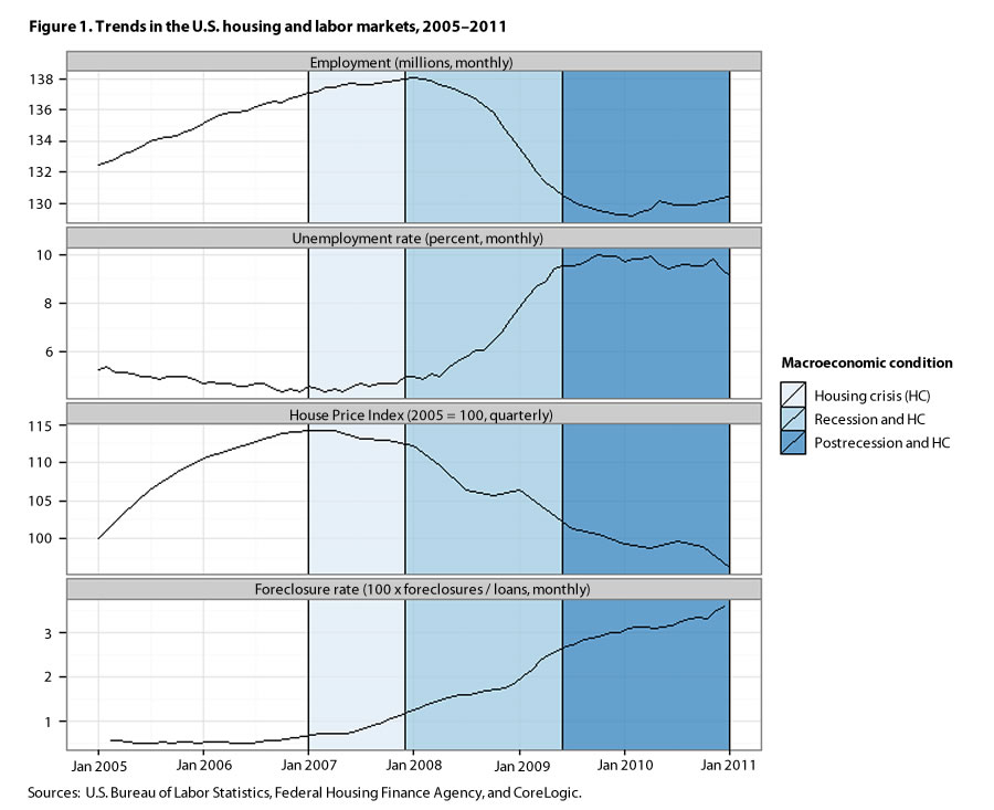
National picture. To provide context for the analysis of MSAs, figure 1 presents information on national U.S. housing and labor market conditions for the period 2005–2011. Housing prices in the nation accelerated during the early to mid-2000s and, according to the FHFA House Price Index, reached a peak in first quarter 2007.31 From 2007 to 2010, housing prices declined nearly 13 percent on average in the United States, and the foreclosure rate—a measure of acute housing distress—rose from 0.87 percent to 3.26 percent, a whopping 274-percent increase.32 Trends in U.S. employment and unemployment are mirror images and both show a downturn in the labor market by the end of 2007 or early 2008. From 2007 to 2010, the unemployment rate rose from 4.6 percent to 9.6 percent, while employment fell by 5.6 percent. The data also show that the Great Recession’s start date of December 2007, as determined by the National Bureau of Economic Research, virtually coincides with the start of the labor market downturn. As shown in figure 1, the national situation from 2005 to 2011 can be described as having progressed through four distinct periods: the precrisis period (before 2007), the housing-crisis-only period (first quarter 2007–end of 2007), the housing recession period (end of 2007–summer 2009), and the postrecession period (after summer 2009). As of the end of 2012, the national unemployment rate remained only slightly below 8 percent.
In terms of the timing of the housing and labor market crises, figure 1 shows the well-known story for the United States: the start of the housing crisis, as defined by the fall in housing prices, preceded the downturn in the labor market. This is also the sequence of events for a number of the largest, but not the majority of, MSAs.

| Year | Variable | Value |
|---|---|---|
| 2005 | Employment (millions) | 113.836 |
| 2006 | Employment (millions) | 115.440 |
| 2007 | Employment (millions) | 116.762 |
| 2008 | Employment (millions) | 116.655 |
| 2009 | Employment (millions) | 112.369 |
| 2010 | Employment (millions) | 112.195 |
| 2005 | House Price Index (2005 = 100) | 100.00 |
| 2006 | House Price Index (2005 = 100) | 105.75 |
| 2007 | House Price Index (2005 = 100) | 107.16 |
| 2008 | House Price Index (2005 = 100) | 102.35 |
| 2009 | House Price Index (2005 = 100) | 97.42 |
| 2010 | House Price Index (2005 = 100) | 93.84 |
| 2005 | Foreclosure rate (100 x foreclosures / loans) | .51 |
| 2006 | Foreclosure rate (100 x foreclosures / loans) | .55 |
| 2007 | Foreclosure rate (100 x foreclosures / loans) | .87 |
| 2008 | Foreclosure rate (100 x foreclosures / loans) | 1.59 |
| 2009 | Foreclosure rate (100 x foreclosures / loans) | 2.65 |
| 2010 | Foreclosure rate (100 x foreclosures / loans) | 3.26 |
| 2005 | Homeownership rate (percent) | 66.27 |
| 2006 | Homeownership rate (percent) | 66.70 |
| 2007 | Homeownership rate (percent) | 66.63 |
| 2008 | Homeownership rate (percent) | 66.10 |
| 2009 | Homeownership rate (percent) | 64.58 |
| 2010 | Homeownership rate (percent) | 63.93 |
| 2005 | Household size | 3.57 |
| 2006 | Household size | 3.61 |
| 2007 | Household size | 3.61 |
| 2008 | Household size | 3.64 |
| 2009 | Household size | 3.67 |
| 2010 | Household size | 3.65 |
| 2005 | Nonrelatives in family households (percent) | 2.37 |
| 2006 | Nonrelatives in family households (percent) | 2.51 |
| 2007 | Nonrelatives in family households (percent) | 2.52 |
| 2008 | Nonrelatives in family households (percent) | 2.45 |
| 2009 | Nonrelatives in family households (percent) | 2.61 |
| 2010 | Nonrelatives in family households (percent) | 2.75 |
| 2005 | Unmarried households (percent) | 7.40 |
| 2006 | Unmarried households (percent) | 7.44 |
| 2007 | Unmarried households (percent) | 7.61 |
| 2008 | Unmarried households (percent) | 7.62 |
| 2009 | Unmarried households (percent) | 7.91 |
| 2010 | Unmarried households (percent) | 8.22 |
| Sources: U.S. Bureau of Labor Statistics, Federal Housing Finance Agency, CoreLogic, American Community Survey, and authors’ calculations. | ||
MSA-level picture: an overview. Figure 2 illustrates annual trends in employment and housing conditions for all 353 MSAs (unweighted) for the period 2005–2010. These trends closely match those for the nation (MSAs weighted by population size) reported in figure 1. Most notably, figure 2 again shows that the housing crisis started first, followed by the labor market crisis. The top panel of table 2 provides annual statistics for 2 specific years shown in figure 2—2007 and 2010. Statistics are presented for 2007 rather than for 2005 because most MSAs had experienced rising employment and housing prices even before 2007.33 Table 2 shows that, between 2007 and 2010, housing prices fell on average by nearly 10 percent across the 353 MSAs. This average decline is slightly lower than that for the nation as a whole (see figure 1), because these estimates are unweighted and thereby reflect the fact that housing prices declined less in smaller MSAs.34
| Variable | 2007 | 2010 | Percent change (2007–2010) | |||||||||
|---|---|---|---|---|---|---|---|---|---|---|---|---|
| Mean | Standard deviation | Minimum | Median | Maximum | Mean | Standard deviation | Minimum | Median | Maximum | Mean | Median | |
| All 353 MSAs | ||||||||||||
| Employment (thousands) | 325.2 | 573.6 | 29.1 | 123.5 | 5,304.2 | 312.5 | 549.8 | 28.6 | 116.7 | 5,153.7 | –4.07 | –5.52 |
| House Price Index | 108.2 | 8.0 | 90.6 | 107.3 | 137.3 | 98.4 | 16.9 | 41.5 | 103.1 | 148.5 | –9.97 | –3.92 |
| Foreclosure rate (percent) | .80 | .50 | .11 | .67 | 3.07 | 2.51 | 2.23 | .49 | 1.93 | 17.71 | 68.11 | 190.34 |
| Homeownership rate (percent) | 68.00 | 5.73 | 40.96 | 68.92 | 82.68 | 66.41 | 6.06 | 39.53 | 67.15 | 81.46 | –2.40 | –2.58 |
| Household size | 3.50 | .23 | 2.63 | 3.48 | 4.32 | 3.56 | .21 | 3.06 | 3.55 | 4.40 | 1.54 | 1.98 |
| Nonrelatives in family households (percent) | 2.49 | .71 | .89 | 2.37 | 4.75 | 2.69 | .72 | 1.07 | 2.60 | 5.87 | 7.37 | 9.38 |
| Unmarried households (percent) | 7.75 | 1.87 | 2.16 | 7.80 | 14.88 | 8.22 | 1.89 | 1.66 | 8.17 | 13.88 | 5.72 | 4.79 |
| Housing crisis first MSAs (55 MSAs) | ||||||||||||
| Employment (thousands) | 576.8 | 850.7 | 29.1 | 210.9 | 5,304.2 | 559.2 | 828.2 | 28.6 | 201.6 | 5,153.7 | –3.15 | –4.42 |
| House Price Index | 103.4 | 8.0 | 90.7 | 103.9 | 137.3 | 78.0 | 17.7 | 41.5 | 81.5 | 124.7 | –32.60 | –21.53 |
| Foreclosure rate (percent) | .87 | .48 | .12 | .80 | 2.09 | 3.60 | 2.57 | .82 | 2.80 | 13.20 | 75.96 | 251.48 |
| Homeownership rate (percent) | 65.28 | 8.03 | 40.96 | 65.83 | 82.68 | 63.20 | 7.79 | 39.53 | 63.42 | 81.46 | –3.29 | –3.66 |
| Household size | 3.63 | .26 | 3.08 | 3.63 | 4.19 | 3.69 | .22 | 3.25 | 3.66 | 4.24 | 1.43 | .67 |
| Nonrelatives in family households (percent) | 2.82 | .66 | 1.80 | 2.80 | 4.48 | 3.25 | .78 | 1.79 | 3.10 | 5.87 | 13.31 | 11.05 |
| Unmarried households (percent) | 8.12 | 1.45 | 5.06 | 7.98 | 11.08 | 8.49 | 1.59 | 5.25 | 8.40 | 11.84 | 4.30 | 5.30 |
| Labor market crisis first MSAs (67 MSAs) | ||||||||||||
| Employment (thousands) | 142.3 | 247.9 | 39.1 | 74.5 | 1,968.8 | 137.9 | 248.8 | 37.3 | 71.1 | 1,987.9 | –3.19 | –4.57 |
| House Price Index | 107.9 | 3.8 | 102.5 | 107.2 | 122.2 | 107.8 | 5.5 | 93.8 | 107.8 | 123.3 | –.10 | .57 |
| Foreclosure rate (percent) | .74 | .40 | .25 | .62 | 2.37 | 1.62 | .64 | .67 | 1.51 | 3.96 | 54.29 | 144.68 |
| Homeownership rate (percent) | 68.09 | 4.57 | 54.55 | 68.51 | 75.22 | 66.47 | 5.63 | 48.21 | 67.41 | 76.74 | –2.43 | –1.61 |
| Household size | 3.44 | .19 | 3.08 | 3.43 | 4.03 | 3.51 | .19 | 3.06 | 3.52 | 4.20 | 2.16 | 2.69 |
| Nonrelatives in family households (percent) | 2.35 | .69 | 1.22 | 2.28 | 4.40 | 2.47 | .57 | 1.23 | 2.38 | 4.16 | 4.87 | 4.50 |
| Unmarried households (percent) | 6.97 | 2.06 | 2.45 | 6.93 | 12.30 | 7.87 | 1.81 | 3.49 | 8.03 | 12.45 | 11.37 | 15.89 |
| Notes: Note: These data are unweighted. "Housing crisis first" MSAs are those where the housing market turned downward four or more quarters before the labor market did; "labor market crisis first" MSAs are those where the labor market turned downward four or more quarters before the housing market did. Omitted MSAs are those where the housing and labor market crises occurred "concurrently" (defined as less than four quarters difference in timing) and those where peaks could not be clearly identified. Sources: U.S. Bureau of Labor Statistics, Federal Housing Finance Agency, CoreLogic, American Community Survey, and authors' calculations. | ||||||||||||
Figure 2 and the top panel of table 2 also provide information on annual trends in homeownership rates, measures of doubling up, and the percentage of unmarried households for the 353 MSAs. Consistent with the research on national trends cited earlier, the figure and the table show that doubling up increased, whether measured by higher average household size or by nonrelatives as a percentage of all individuals living in family households. The fraction of unmarried households also rose over the period 2007–2010, in part because of the rising secular trend, but also because of weak economic conditions.35 Finally, table 2 shows that homeownership rates fell in conjunction with both the decline in housing prices and the rise in foreclosures. Although suggestive, these aggregate data mask substantial subnational variation in the severity, duration, and timing of the crises; these data also obscure the considerable heterogeneity in changes in doubling up and homeownership at the subnational level.
MSA-level analysis: timing of the housing and labor market crises. The analysis identifies the start of each crisis by examining quarterly data from 2005 to 2011. A crisis in the housing market is identified when housing prices, a measure of overall housing conditions, peak in a given quarter and then turn downward.36 Similarly, a crisis in the labor market is identified when employment peaks in a given quarter and then falls. In the case that either the housing price or the employment series has multiple peaks, the peak used is the one that precedes the longest downturn.37
| Number of MSAs | Difference in timing (in number of quarters)(1) |
|---|---|
0 | –22.9 |
1 | –21.9 |
0 | –20.8 |
2 | –19.7 |
0 | –18.7 |
0 | –17.6 |
1 | –16.5 |
4 | –15.5 |
1 | –14.4 |
3 | –13.3 |
3 | –12.3 |
7 | –11.2 |
12 | –10.1 |
12 | –9.1 |
11 | –8.0 |
7 | –6.9 |
11 | –5.9 |
12 | –4.8 |
17 | –3.7 |
33 | –2.7 |
15 | –1.6 |
26 | –0.5 |
48 | 0.5 |
28 | 1.6 |
33 | 2.7 |
22 | 3.7 |
10 | 4.8 |
10 | 5.9 |
15 | 6.9 |
1 | 8.0 |
7 | 9.1 |
2 | 10.1 |
0 | 11.2 |
| Notes: (1) Positive values indicate that the housing market crisis occurred first. | |
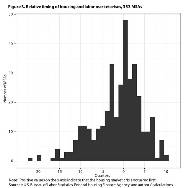
Figure 3 provides a histogram of the relative timing of the crises for the 353 MSAs, where differences in timing are measured in number of quarters. A positive value indicates that the housing market crisis occurred first, whereas a negative value indicates that the labor market crisis occurred first. The distribution is slightly skewed to the left, indicating that in a slight majority of MSAs, it was the labor market, not the housing market, that turned downward first. This pattern is contrary to the one for the nation as a whole. (See figure 1.) The reason for the difference is that the national picture is driven by timing patterns in the largest MSAs.
To illustrate this point, table 3 provides information on the relative timing of the housing and labor market crises for the 25 largest MSAs (based on employment size). In 20 of the 25 MSAs, the housing market declined first, and in 10 of these 20 MSAs, the housing market declined four or more quarters earlier. In 5 of the 25 MSAs, the labor market declined first, and only Dallas experienced a decline of four or more quarters. Table 3 also shows that the timing of the start of the housing crisis for the largest MSAs is fairly close to the timing for the nation as a whole. (See also figures 1 and 2.) The MSAs identified in yellow in the table receive greater attention shortly.
| MSA | Rank by employment size | Onset of housing market crisis | Onset of labor market crisis | Housing market crisis before labor market crisis (in number of quarters)(1) |
|---|---|---|---|---|
| New York–White Plains–Wayne, NY–NJ Metro Division; New York–Northern New Jersey–Long Island, NY–NJ–PA Metro Area | 1 | 1st quarter, 2007 | 1st quarter, 2008 | 4 |
| Los Angeles–Long Beach–Santa Ana, CA Metro Area | 2 | 4th quarter, 2006 | 3rd quarter, 2007 | 3 |
| Chicago–Joliet–Naperville, IL–IN–WI Metro Area | 3 | 1st quarter, 2007 | 4th quarter, 2007 | 3 |
| Houston–Sugar Land–Baytown, TX Metro Area | 4 | 2nd quarter, 2009 | 4th quarter, 2008 | –2 |
| Atlanta–Sandy Springs–Marietta, GA Metro Area | 5 | 3rd quarter, 2007 | 4th quarter, 2007 | 1 |
| Washington–Arlington–Alexandria, DC–VA–MD–WV Metro Area | 6 | 4th quarter, 2006 | 3rd quarter, 2008 | 7 |
| Dallas–Fort Worth–Arlington, TX Metro Area | 7 | 1st quarter, 2009 | 1st quarter, 2008 | –4 |
| Phoenix–Mesa–Glendale, AZ Metro Area | 8 | 4th quarter, 2006 | 1st quarter, 2008 | 5 |
| Philadelphia–Camden–Wilmington, PA–NJ–DE–MD Metro Area | 9 | 3rd quarter, 2007 | 2nd quarter, 2008 | 3 |
| Minneapolis–St. Paul–Bloomington, MN–WI Metro Area | 10 | 4th quarter, 2006 | 2nd quarter, 2008 | 6 |
| Riverside–San Bernardino–Ontario, CA Metro Area | 11 | 4th quarter, 2006 | 1st quarter, 2007 | 1 |
| Los Angeles–Long Beach–Santa Ana, CA Metro Area | 12 | 3rd quarter, 2006 | 4th quarter, 2006 | 1 |
| San Diego–Carlsbad–San Marcos, CA Metro Area | 13 | 1st quarter, 2006 | 2nd quarter, 2008 | 9 |
| Boston–Cambridge–Quincy, MA–NH Metro Area | 14 | 4th quarter, 2005 | 2nd quarter, 2008 | 10 |
| Nassau–Suffolk, NY Metro Division; New York–Northern New Jersey–Long Island, NY–NJ–PA Metro Area | 15 | 4th quarter, 2006 | 1st quarter, 2008 | 5 |
| St. Louis, MO–IL Metro Area | 16 | 3rd quarter, 2007 | 1st quarter, 2007 | –2 |
| Baltimore–Towson, MD Metro Area | 17 | 2nd quarter, 2007 | 1st quarter, 2008 | 3 |
| Seattle–Tacoma–Bellevue, WA Metro Area | 18 | 3rd quarter, 2007 | 2nd quarter, 2008 | 3 |
| Denver–Aurora–Broomfield, CO Metro Area | 19 | 4th quarter, 2006 | 2nd quarter, 2008 | 6 |
| Detroit–Warren–Livonia, MI Metro Area | 20 | 3rd quarter, 2005 | 2nd quarter, 2005 | –1 |
| Tampa–St. Petersburg–Clearwater, FL Metro Area | 21 | 4th quarter, 2006 | 2nd quarter, 2007 | 2 |
| San Francisco–Oakland–Fremont, CA Metro Area | 22 | 2nd quarter, 2006 | 1st quarter, 2008 | 7 |
| Pittsburgh, PA Metro Area | 23 | 2nd quarter, 2009 | 3rd quarter, 2008 | –3 |
| Edison–New Brunswick, NJ Metro Division; New York–Northern New Jersey–Long Island, NY–NJ–PA Metro Area | 24 | 4th quarter, 2006 | 1st quarter, 2008 | 5 |
| Miami–Fort Lauderdale–Pompano Beach, FL Metro Area | 25 | 2nd quarter, 2007 | 4th quarter, 2007 | 2 |
| Notes: (1) Positive values indicate that the housing market declined first; negative values indicate that the labor market declined first. | ||||
Next, the analysis uses a “four-quarter rule” to identify the MSAs that had clearly different experiences regarding the timing of the crises. MSAs are categorized as “housing crisis first” if the housing market turned downward four or more quarters before the labor market did. MSAs are categorized as “labor market crisis first” if the labor market turned downward four or more quarters before the housing market did. As found earlier, the number of MSAs in which the labor market crisis occurred first was slightly larger than the number of MSAs in which the housing market crisis occurred first: 67 versus 55, respectively.38
| MSA ID | Name | Housing market crisis before labor market crisis (in number of quarters) |
|---|---|---|
10180 | Abilene, TX Metro Area | 1 |
10420 | Akron, OH Metro Area | 9 |
10500 | Albany, GA Metro Area | –2 |
10580 | Albany–Schenectady–Troy, NY Metro Area | 1 |
10740 | Albuquerque, NM Metro Area | 0 |
10780 | Alexandria, LA Metro Area | –8 |
10900 | Allentown–Bethlehem–Easton, PA–NJ Metro Area | 3 |
11020 | Altoona, PA Metro Area | –7 |
11100 | Amarillo, TX Metro Area | –15 |
11180 | Ames, IA Metro Area | –8 |
11260 | Anchorage, AK Metro Area | –1 |
11300 | Anderson, IN Metro Area | –1 |
11340 | Anderson, SC Metro Area | –3 |
11460 | Ann Arbor, MI Metro Area | 2 |
11500 | Anniston–Oxford, AL Metro Area | –10 |
11540 | Appleton, WI Metro Area | 2 |
11700 | Asheville, NC Metro Area | 0 |
12020 | Athens–Clarke County, GA Metro Area | 0 |
12060 | Atlanta–Sandy Springs–Marietta, GA Metro Area | 1 |
12100 | Atlantic City–Hammonton, NJ Metro Area | 4 |
12220 | Auburn–Opelika, AL Metro Area | –3 |
12260 | Augusta–Richmond County, GA–SC Metro Area | –3 |
12540 | Bakersfield–Delano, CA Metro Area | 7 |
12580 | Baltimore–Towson, MD Metro Area | 3 |
12940 | Baton Rouge, LA Metro Area | –3 |
12980 | Battle Creek, MI Metro Area | –3 |
13020 | Bay City, MI Metro Area | 3 |
13140 | Beaumont–Port Arthur, TX Metro Area | –3 |
13380 | Bellingham, WA Metro Area | 2 |
13460 | Bend, OR Metro Area | 2 |
13644 | Bethesda–Rockville–Frederick, MD Metro Division; Washington–Arlington–Alexandria, DC–VA–MD–WV Metro Area | 6 |
13740 | Billings, MT Metro Area | –4 |
13780 | Binghamton, NY Metro Area | –9 |
13820 | Birmingham–Hoover, AL Metro Area | –8 |
13900 | Bismarck, ND Metro Area | 1 |
13980 | Blacksburg–Christiansburg–Radford, VA Metro Area | –1 |
14020 | Bloomington, IN Metro Area | –9 |
14060 | Bloomington–Normal, IL Metro Area | –12 |
14260 | Boise City–Nampa, ID Metro Area | –1 |
14484 | Boston–Quincy, MA Metro Division; Boston–Cambridge–Quincy, MA–NH Metro Area | 10 |
14500 | Boulder, CO Metro Area | –4 |
14540 | Bowling Green, KY Metro Area | –5 |
14740 | Bremerton–Silverdale, WA Metro Area | 3 |
15180 | Brownsville–Harlingen, TX Metro Area | –10 |
15260 | Brunswick, GA Metro Area | 1 |
15380 | Buffalo–Niagara Falls, NY Metro Area | –11 |
15500 | Burlington, NC Metro Area | –5 |
15804 | Camden, NJ Metro Division; Philadelphia–Camden–Wilmington, PA–NJ–DE–MD Metro Area | 3 |
15940 | Canton–Massillon, OH Metro Area | 9 |
15980 | Cape Coral–Fort Myers, FL Metro Area | 3 |
16020 | Cape Girardeau–Jackson, MO–IL Metro Area | –7 |
16220 | Casper, WY Metro Area | 2 |
16300 | Cedar Rapids, IA Metro Area | –8 |
16580 | Champaign–Urbana, IL Metro Area | –10 |
16620 | Charleston, WV Metro Area | –10 |
16700 | Charleston–North Charleston–Summerville, SC Metro Area | 1 |
16740 | Charlotte–Gastonia–Rock Hill, NC–SC Metro Area | 0 |
16820 | Charlottesville, VA Metro Area | 4 |
16860 | Chattanooga, TN–GA Metro Area | –13 |
16940 | Cheyenne, WY Metro Area | –3 |
16974 | Chicago–Joliet–Naperville, IL Metro Division; Chicago–Joliet–Naperville, IL–IN–WI Metro Area | 3 |
17020 | Chico, CA Metro Area | 7 |
17140 | Cincinnati–Middletown, OH–KY–IN Metro Area | 4 |
17300 | Clarksville, TN–KY Metro Area | –13 |
17420 | Cleveland, TN Metro Area | –9 |
17460 | Cleveland–Elyria–Mentor, OH Metro Area | 5 |
17780 | College Station–Bryan, TX Metro Area | 0 |
17820 | Colorado Springs, CO Metro Area | 3 |
17860 | Columbia, MO Metro Area | –3 |
17900 | Columbia, SC Metro Area | –6 |
17980 | Columbus, GA–AL Metro Area | –4 |
18020 | Columbus, IN Metro Area | –3 |
18140 | Columbus, OH Metro Area | 5 |
18580 | Corpus Christi, TX Metro Area | –16 |
18700 | Corvallis, OR Metro Area | 1 |
19060 | Cumberland, MD–WV Metro Area | –3 |
19124 | Dallas–Plano–Irving, TX Metro Division; Dallas–Fort Worth–Arlington, TX Metro Area | –4 |
19140 | Dalton, GA Metro Area | –10 |
19180 | Danville, IL Metro Area | –3 |
19260 | Danville, VA Metro Area | –15 |
19340 | Davenport–Moline–Rock Island, IA–IL Metro Area | –5 |
19380 | Dayton, OH Metro Area | –2 |
19460 | Decatur, AL Metro Area | –11 |
19500 | Decatur, IL Metro Area | –6 |
19660 | Deltona–Daytona Beach–Ormond Beach, FL Metro Area | 3 |
19740 | Denver–Aurora–Broomfield, CO Metro Area | 6 |
19780 | Des Moines–West Des Moines, IA Metro Area | 2 |
19804 | Detroit–Livonia–Dearborn, MI Metro Division; Detroit–Warren–Livonia, MI Metro Area | –1 |
20020 | Dothan, AL Metro Area | –8 |
20100 | Dover, DE Metro Area | 1 |
20260 | Duluth, MN–WI Metro Area | 2 |
20500 | Durham–Chapel Hill, NC Metro Area | –1 |
20740 | Eau Claire, WI Metro Area | 0 |
20764 | Edison–New Brunswick, NJ Metro Division; New York–Northern New Jersey–Long Island, NY–NJ–PA Metro Area | 5 |
20940 | El Centro, CA Metro Area | 7 |
21060 | Elizabethtown, KY Metro Area | –1 |
21140 | Elkhart–Goshen, IN Metro Area | –6 |
21300 | Elmira, NY Metro Area | –6 |
21340 | El Paso, TX Metro Area | –9 |
21500 | Erie, PA Metro Area | –10 |
21660 | Eugene–Springfield, OR Metro Area | 2 |
21780 | Evansville, IN–KY Metro Area | 1 |
21820 | Fairbanks, AK Metro Area | 2 |
22020 | Fargo, ND–MN Metro Area | –4 |
22140 | Farmington, NM Metro Area | –3 |
22180 | Fayetteville, NC Metro Area | –11 |
22220 | Fayetteville–Springdale–Rogers, AR–MO Metro Area | 4 |
22380 | Flagstaff, AZ Metro Area | 6 |
22420 | Flint, MI Metro Area | 1 |
22500 | Florence, SC Metro Area | –5 |
22520 | Florence–Muscle Shoals, AL Metro Area | –8 |
22540 | Fond du Lac, WI Metro Area | 1 |
22660 | Fort Collins–Loveland, CO Metro Area | 3 |
22744 | Fort Lauderdale–Pompano Beach–Deerfield Beach, FL Metro Division; Miami–Fort Lauderdale–Pompano Beach, FL Metro Area | 3 |
22900 | Fort Smith, AR–OK Metro Area | –6 |
23060 | Fort Wayne, IN Metro Area | –1 |
23104 | Fort Worth–Arlington, TX Metro Division; Dallas–Fort Worth–Arlington, TX Metro Area | –3 |
23420 | Fresno, CA Metro Area | 6 |
23460 | Gadsden, AL Metro Area | –10 |
23540 | Gainesville, FL Metro Area | 3 |
23580 | Gainesville, GA Metro Area | 1 |
23844 | Gary, IN Metro Division; Chicago–Joliet–Naperville, IL–IN–WI Metro Area | 1 |
24020 | Glens Falls, NY Metro Area | –2 |
24140 | Goldsboro, NC Metro Area | –5 |
24220 | Grand Forks, ND–MN Metro Area | –9 |
24300 | Grand Junction, CO Metro Area | 1 |
24340 | Grand Rapids–Wyoming, MI Metro Area | 3 |
24500 | Great Falls, MT Metro Area | 5 |
24540 | Greeley, CO Metro Area | 10 |
24580 | Green Bay, WI Metro Area | –1 |
24660 | Greensboro–High Point, NC Metro Area | –3 |
24780 | Greenville, NC Metro Area | –9 |
24860 | Greenville–Mauldin–Easley, SC Metro Area | –4 |
25060 | Gulfport–Biloxi, MS Metro Area | 1 |
25180 | Hagerstown–Martinsburg, MD–WV Metro Area | 4 |
25260 | Hanford–Corcoran, CA Metro Area | 7 |
25420 | Harrisburg–Carlisle, PA Metro Area | 0 |
25500 | Harrisonburg, VA Metro Area | 0 |
25620 | Hattiesburg, MS Metro Area | –2 |
25860 | Hickory–Lenoir–Morganton, NC Metro Area | –10 |
26100 | Holland–Grand Haven, MI Metro Area | –1 |
26180 | Honolulu, HI Metro Area | 2 |
26300 | Hot Springs, AR Metro Area | –3 |
26380 | Houma–Bayou Cane–Thibodaux, LA Metro Area | –9 |
26420 | Houston–Sugar Land–Baytown, TX Metro Area | –2 |
26580 | Huntington–Ashland, WV–KY–OH Metro Area | –7 |
26620 | Huntsville, AL Metro Area | –5 |
26820 | Idaho Falls, ID Metro Area | –1 |
26900 | Indianapolis–Carmel, IN Metro Area | 1 |
26980 | Iowa City, IA Metro Area | –3 |
27060 | Ithaca, NY Metro Area | –7 |
27100 | Jackson, MI Metro Area | 0 |
27140 | Jackson, MS Metro Area | –5 |
27180 | Jackson, TN Metro Area | –7 |
27260 | Jacksonville, FL Metro Area | 2 |
27340 | Jacksonville, NC Metro Area | 0 |
27500 | Janesville, WI Metro Area | –5 |
27620 | Jefferson City, MO Metro Area | –14 |
27740 | Johnson City, TN Metro Area | –4 |
27780 | Johnstown, PA Metro Area | –3 |
27860 | Jonesboro, AR Metro Area | –11 |
27900 | Joplin, MO Metro Area | –9 |
28020 | Kalamazoo–Portage, MI Metro Area | 0 |
28100 | Kankakee–Bradley, IL Metro Area | –1 |
28140 | Kansas City, MO–KS Metro Area | 0 |
28420 | Kennewick–Pasco–Richland, WA Metro Area | –22 |
28660 | Killeen–Temple–Fort Hood, TX Metro Area | –17 |
28700 | Kingsport–Bristol–Bristol, TN–VA Metro Area | –3 |
28740 | Kingston, NY Metro Area | –1 |
28940 | Knoxville, TN Metro Area | –6 |
29020 | Kokomo, IN Metro Area | –1 |
29100 | La Crosse, WI–MN Metro Area | –1 |
29140 | Lafayette, IN Metro Area | –3 |
29180 | Lafayette, LA Metro Area | –3 |
29340 | Lake Charles, LA Metro Area | –3 |
29404 | Lake County–Kenosha County, IL–WI Metro Division; Chicago–Joliet–Naperville, IL–IN–WI Metro Area | 3 |
29420 | Lake Havasu City–Kingman, AZ Metro Area | 0 |
29460 | Lakeland–Winter Haven, FL Metro Area | 2 |
29540 | Lancaster, PA Metro Area | 1 |
29620 | Lansing–East Lansing, MI Metro Area | 7 |
29700 | Laredo, TX Metro Area | –1 |
29740 | Las Cruces, NM Metro Area | 2 |
29820 | Las Vegas–Paradise, NV Metro Area | 7 |
29940 | Lawrence, KS Metro Area | –5 |
30020 | Lawton, OK Metro Area | –1 |
30140 | Lebanon, PA Metro Area | –4 |
30460 | Lexington–Fayette, KY Metro Area | –4 |
30620 | Lima, OH Metro Area | –9 |
30700 | Lincoln, NE Metro Area | 1 |
30780 | Little Rock–North Little Rock–Conway, AR Metro Area | –2 |
30860 | Logan, UT–ID Metro Area | –3 |
30980 | Longview, TX Metro Area | –7 |
31020 | Longview, WA Metro Area | 0 |
31084 | Los Angeles–Long Beach–Glendale, CA Metro Division; Los Angeles–Long Beach–Santa Ana, CA Metro Area | 3 |
31140 | Louisville/Jefferson County, KY–IN Metro Area | –3 |
31180 | Lubbock, TX Metro Area | –11 |
31340 | Lynchburg, VA Metro Area | –2 |
31420 | Macon, GA Metro Area | 1 |
31460 | Madera–Chowchilla, CA Metro Area | 6 |
31540 | Madison, WI Metro Area | 2 |
31740 | Manhattan, KS Metro Area | 4 |
31860 | Mankato–North Mankato, MN Metro Area | 6 |
31900 | Mansfield, OH Metro Area | –3 |
32780 | Medford, OR Metro Area | 3 |
32820 | Memphis, TN–MS–AR Metro Area | 0 |
32900 | Merced, CA Metro Area | 6 |
33124 | Miami–Miami Beach–Kendall, FL Metro Division; Miami–Fort Lauderdale–Pompano Beach, FL Metro Area | 2 |
33140 | Michigan City–La Porte, IN Metro Area | –4 |
33260 | Midland, TX Metro Area | –2 |
33340 | Milwaukee–Waukesha–West Allis, WI Metro Area | 1 |
33460 | Minneapolis–St. Paul–Bloomington, MN–WI Metro Area | 6 |
33540 | Missoula, MT Metro Area | –4 |
33660 | Mobile, AL Metro Area | –4 |
33700 | Modesto, CA Metro Area | 7 |
33740 | Monroe, LA Metro Area | –6 |
33780 | Monroe, MI Metro Area | 2 |
33860 | Montgomery, AL Metro Area | –3 |
34060 | Morgantown, WV Metro Area | –3 |
34100 | Morristown, TN Metro Area | –4 |
34580 | Mount Vernon–Anacortes, WA Metro Area | 1 |
34620 | Muncie, IN Metro Area | 5 |
34740 | Muskegon–Norton Shores, MI Metro Area | 3 |
34820 | Myrtle Beach–North Myrtle Beach–Conway, SC Metro Area | –1 |
34900 | Napa, CA Metro Area | 8 |
34940 | Naples–Marco Island, FL Metro Area | 1 |
34980 | Nashville–Davidson––Murfreesboro––Franklin, TN Metro Area | –1 |
35004 | Nassau–Suffolk, NY Metro Division; New York–Northern New Jersey–Long Island, NY–NJ–PA Metro Area | 5 |
35084 | Newark–Union, NJ–PA Metro Division; New York–Northern New Jersey–Long Island, NY–NJ–PA Metro Area | 4 |
35380 | New Orleans–Metairie–Kenner, LA Metro Area | –8 |
35644 | New York–White Plains–Wayne, NY–NJ Metro Division; New York–Northern New Jersey–Long Island, NY–NJ–PA Metro Area | 4 |
35660 | Niles–Benton Harbor, MI Metro Area | 0 |
36084 | Oakland–Fremont–Hayward, CA Metro Division; San Francisco–Oakland–Fremont, CA Metro Area | 7 |
36100 | Ocala, FL Metro Area | 1 |
36140 | Ocean City, NJ Metro Area | –1 |
36220 | Odessa, TX Metro Area | –2 |
36260 | Ogden–Clearfield, UT Metro Area | 1 |
36420 | Oklahoma City, OK Metro Area | –20 |
36500 | Olympia, WA Metro Area | 3 |
36540 | Omaha–Council Bluffs, NE–IA Metro Area | 4 |
36740 | Orlando–Kissimmee–Sanford, FL Metro Area | 3 |
36780 | Oshkosh–Neenah, WI Metro Area | 2 |
36980 | Owensboro, KY Metro Area | –6 |
37100 | Oxnard–Thousand Oaks–Ventura, CA Metro Area | 7 |
37340 | Palm Bay–Melbourne–Titusville, FL Metro Area | 4 |
37380 | Palm Coast, FL Metro Area | 4 |
37460 | Panama City–Lynn Haven–Panama City Beach, FL Metro Area | 5 |
37620 | Parkersburg–Marietta–Vienna, WV–OH Metro Area | –12 |
37700 | Pascagoula, MS Metro Area | 2 |
37860 | Pensacola–Ferry Pass–Brent, FL Metro Area | 3 |
37900 | Peoria, IL Metro Area | –10 |
37964 | Philadelphia, PA Metro Division; Philadelphia–Camden–Wilmington, PA–NJ–DE–MD Metro Area | 3 |
38060 | Phoenix–Mesa–Glendale, AZ Metro Area | 5 |
38220 | Pine Bluff, AR Metro Area | –20 |
38300 | Pittsburgh, PA Metro Area | –3 |
38540 | Pocatello, ID Metro Area | –3 |
38900 | Portland–Vancouver–Hillsboro, OR–WA Metro Area | 3 |
38940 | Port St. Lucie, FL Metro Area | 4 |
39100 | Poughkeepsie–Newburgh–Middletown, NY Metro Area | 4 |
39140 | Prescott, AZ Metro Area | 1 |
39340 | Provo–Orem, UT Metro Area | 0 |
39380 | Pueblo, CO Metro Area | 4 |
39460 | Punta Gorda, FL Metro Area | 3 |
39540 | Racine, WI Metro Area | 3 |
39580 | Raleigh–Cary, NC Metro Area | –1 |
39660 | Rapid City, SD Metro Area | –10 |
39740 | Reading, PA Metro Area | 2 |
39820 | Redding, CA Metro Area | 2 |
39900 | Reno–Sparks, NV Metro Area | 5 |
40060 | Richmond, VA Metro Area | 4 |
40140 | Riverside–San Bernardino–Ontario, CA Metro Area | 1 |
40220 | Roanoke, VA Metro Area | –3 |
40340 | Rochester, MN Metro Area | –1 |
40380 | Rochester, NY Metro Area | –10 |
40420 | Rockford, IL Metro Area | –1 |
40580 | Rocky Mount, NC Metro Area | –9 |
40660 | Rome, GA Metro Area | –4 |
40900 | Sacramento––Arden–Arcade––Roseville, CA Metro Area | 4 |
40980 | Saginaw–Saginaw Township North, MI Metro Area | 4 |
41060 | St. Cloud, MN Metro Area | 1 |
41100 | St. George, UT Metro Area | 2 |
41140 | St. Joseph, MO–KS Metro Area | –8 |
41180 | St. Louis, MO–IL Metro Area | –2 |
41420 | Salem, OR Metro Area | 2 |
41500 | Salinas, CA Metro Area | 9 |
41540 | Salisbury, MD Metro Area | 2 |
41620 | Salt Lake City, UT Metro Area | 1 |
41660 | San Angelo, TX Metro Area | –12 |
41740 | San Diego–Carlsbad–San Marcos, CA Metro Area | 9 |
41780 | Sandusky, OH Metro Area | 4 |
41884 | San Francisco–San Mateo–Redwood City, CA Metro Division; San Francisco–Oakland–Fremont, CA Metro Area | 7 |
41940 | San Jose–Sunnyvale–Santa Clara, CA Metro Area | 7 |
42020 | San Luis Obispo–Paso Robles, CA Metro Area | 9 |
42044 | Santa Ana–Anaheim–Irvine, CA Metro Division; Los Angeles–Long Beach–Santa Ana, CA Metro Area | 1 |
42060 | Santa Barbara–Santa Maria–Goleta, CA Metro Area | 9 |
42100 | Santa Cruz–Watsonville, CA Metro Area | 3 |
42140 | Santa Fe, NM Metro Area | –2 |
42220 | Santa Rosa–Petaluma, CA Metro Area | 4 |
42340 | Savannah, GA Metro Area | –1 |
42540 | Scranton––Wilkes–Barre, PA Metro Area | –8 |
42644 | Seattle–Bellevue–Everett, WA Metro Division; Seattle–Tacoma–Bellevue, WA Metro Area | 3 |
43100 | Sheboygan, WI Metro Area | –1 |
43300 | Sherman–Denison, TX Metro Area | –13 |
43580 | Sioux City, IA–NE–SD Metro Area | –5 |
43620 | Sioux Falls, SD Metro Area | –3 |
43780 | South Bend–Mishawaka, IN–MI Metro Area | –6 |
43900 | Spartanburg, SC Metro Area | –4 |
44060 | Spokane, WA Metro Area | 2 |
44180 | Springfield, MO Metro Area | –2 |
44220 | Springfield, OH Metro Area | –3 |
44300 | State College, PA Metro Area | –4 |
44700 | Stockton, CA Metro Area | 3 |
44940 | Sumter, SC Metro Area | –10 |
45060 | Syracuse, NY Metro Area | –8 |
45104 | Tacoma, WA Metro Division; Seattle–Tacoma–Bellevue, WA Metro Area | 3 |
45220 | Tallahassee, FL Metro Area | 3 |
45300 | Tampa–St. Petersburg–Clearwater, FL Metro Area | 2 |
45460 | Terre Haute, IN Metro Area | –3 |
45500 | Texarkana, TX–Texarkana, AR Metro Area | –2 |
45780 | Toledo, OH Metro Area | 4 |
45820 | Topeka, KS Metro Area | –15 |
45940 | Trenton–Ewing, NJ Metro Area | 7 |
46060 | Tucson, AZ Metro Area | 7 |
46140 | Tulsa, OK Metro Area | –9 |
46220 | Tuscaloosa, AL Metro Area | –7 |
46340 | Tyler, TX Metro Area | –2 |
46540 | Utica–Rome, NY Metro Area | –11 |
46660 | Valdosta, GA Metro Area | –5 |
46700 | Vallejo–Fairfield, CA Metro Area | 6 |
47020 | Victoria, TX Metro Area | –2 |
47220 | Vineland–Millville–Bridgeton, NJ Metro Area | 2 |
47260 | Virginia Beach–Norfolk–Newport News, VA–NC Metro Area | 3 |
47300 | Visalia–Porterville, CA Metro Area | 7 |
47380 | Waco, TX Metro Area | –11 |
47580 | Warner Robins, GA Metro Area | 9 |
47644 | Warren–Troy–Farmington Hills, MI Metro Division; Detroit–Warren–Livonia, MI Metro Area | –1 |
47894 | Washington–Arlington–Alexandria, DC–VA–MD–WV Metro Division; Washington–Arlington–Alexandria, DC–VA–MD–WV Metro Area | 7 |
47940 | Waterloo–Cedar Falls, IA Metro Area | –4 |
48140 | Wausau, WI Metro Area | –6 |
48300 | Wenatchee–East Wenatchee, WA Metro Area | 6 |
48424 | West Palm Beach–Boca Raton–Boynton Beach, FL Metro Division; Miami–Fort Lauderdale–Pompano Beach, FL Metro Area | 3 |
48540 | Wheeling, WV–OH Metro Area | –5 |
48620 | Wichita, KS Metro Area | –9 |
48660 | Wichita Falls, TX Metro Area | –6 |
48700 | Williamsport, PA Metro Area | –3 |
48864 | Wilmington, DE–MD–NJ Metro Division; Philadelphia–Camden–Wilmington, PA–NJ–DE–MD Metro Area | 2 |
48900 | Wilmington, NC Metro Area | 3 |
49020 | Winchester, VA–WV Metro Area | 1 |
49180 | Winston–Salem, NC Metro Area | –8 |
49420 | Yakima, WA Metro Area | 0 |
49620 | York–Hanover, PA Metro Area | 2 |
49660 | Youngstown–Warren–Boardman, OH–PA Metro Area | 3 |
49700 | Yuba City, CA Metro Area | 4 |
49740 | Yuma, AZ Metro Area | 5 |
Sources: U.S. Bureau of Labor Statistics, Federal Housing Finance Agency, and authors' claculations. | ||
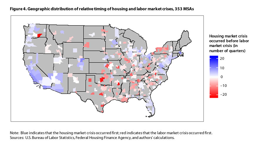
Figure 4 superimposes the 353 MSAs on a map of the United States and illustrates geographic differences in the relative timing of the crises. Blue indicates that the housing crisis occurred first, and red indicates that the labor market crisis occurred first. A visual comparison of the darkest red and darkest blue MSAs provides the clearest indication of the distinct geographic differences in the crises’ relative timing. What is most apparent is that a larger number of MSAs on the coasts experienced the housing crisis first (more blue), whereas more MSAs in the central part of the United States, including Texas, experienced the labor market crisis first (more red). The observed bifurcation by geographic region matches the findings of earlier studies that looked at the magnitude of regional housing bubbles and subsequent bursts.39
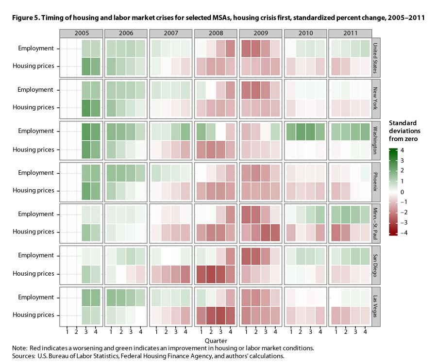
The analysis next looks at the experience of 12 selected MSAs. From the set of “housing crisis first” MSAs, the largest five MSAs (by employment) were selected: these are the MSAs that encompass New York City; Washington, DC; Phoenix; Minneapolis–St. Paul; and San Diego. Although not one of the largest MSAs of this type, Las Vegas was included given the considerable media attention it has received. From the set of “labor market crisis first” MSAs, the largest six were chosen: Dallas, Buffalo, Birmingham, Columbia, Knoxville, and Greenville. The only apparent difference between these two lists is that MSAs where the housing crisis occurred first are considerably larger, with the single exception of Dallas.40
| MSA ID | City | Date | Variable | Standard deviations from zero |
|---|---|---|---|---|
0 | United States | August 15, 2005 | Employment | 1.02 |
29820 | Las Vegas | August 15, 2005 | Employment | 1.72 |
33460 | Minn.–St. Paul | August 15, 2005 | Employment | .48 |
35644 | New York | August 15, 2005 | Employment | 1.35 |
38060 | Phoenix | August 15, 2005 | Employment | 1.54 |
41740 | San Diego | August 15, 2005 | Employment | .33 |
47894 | Washington | August 15, 2005 | Employment | 2.51 |
0 | United States | November 15, 2005 | Employment | .99 |
29820 | Las Vegas | November 15, 2005 | Employment | 1.69 |
33460 | Minn.–St. Paul | November 15, 2005 | Employment | .45 |
35644 | New York | November 15, 2005 | Employment | 1.38 |
38060 | Phoenix | November 15, 2005 | Employment | 1.63 |
41740 | San Diego | November 15, 2005 | Employment | .28 |
47894 | Washington | November 15, 2005 | Employment | 2.17 |
0 | United States | February 14, 2006 | Employment | .93 |
29820 | Las Vegas | February 14, 2006 | Employment | 1.64 |
33460 | Minn.–St. Paul | February 14, 2006 | Employment | .41 |
35644 | New York | February 14, 2006 | Employment | 1.22 |
38060 | Phoenix | February 14, 2006 | Employment | 1.59 |
41740 | San Diego | February 14, 2006 | Employment | .29 |
47894 | Washington | February 14, 2006 | Employment | 1.78 |
0 | United States | May 16, 2006 | Employment | 1.00 |
29820 | Las Vegas | May 16, 2006 | Employment | 1.54 |
33460 | Minn.–St. Paul | May 16, 2006 | Employment | .37 |
35644 | New York | May 16, 2006 | Employment | 1.14 |
38060 | Phoenix | May 16, 2006 | Employment | 1.56 |
41740 | San Diego | May 16, 2006 | Employment | .66 |
47894 | Washington | May 16, 2006 | Employment | 1.70 |
0 | United States | August 15, 2006 | Employment | 1.06 |
29820 | Las Vegas | August 15, 2006 | Employment | 1.30 |
33460 | Minn.–St. Paul | August 15, 2006 | Employment | .42 |
35644 | New York | August 15, 2006 | Employment | 1.12 |
38060 | Phoenix | August 15, 2006 | Employment | 1.44 |
41740 | San Diego | August 15, 2006 | Employment | .91 |
47894 | Washington | August 15, 2006 | Employment | 1.47 |
0 | United States | November 15, 2006 | Employment | .87 |
29820 | Las Vegas | November 15, 2006 | Employment | .93 |
33460 | Minn.–St. Paul | November 15, 2006 | Employment | .21 |
35644 | New York | November 15, 2006 | Employment | .91 |
38060 | Phoenix | November 15, 2006 | Employment | 1.11 |
41740 | San Diego | November 15, 2006 | Employment | .67 |
47894 | Washington | November 15, 2006 | Employment | .91 |
0 | United States | February 14, 2007 | Employment | .59 |
29820 | Las Vegas | February 14, 2007 | Employment | .61 |
33460 | Minn.–St. Paul | February 14, 2007 | Employment | –.04 |
35644 | New York | February 14, 2007 | Employment | .63 |
38060 | Phoenix | February 14, 2007 | Employment | .78 |
41740 | San Diego | February 14, 2007 | Employment | .33 |
47894 | Washington | February 14, 2007 | Employment | .51 |
0 | United States | May 16, 2007 | Employment | .32 |
29820 | Las Vegas | May 16, 2007 | Employment | .39 |
33460 | Minn.–St. Paul | May 16, 2007 | Employment | –.29 |
35644 | New York | May 16, 2007 | Employment | .43 |
38060 | Phoenix | May 16, 2007 | Employment | .55 |
41740 | San Diego | May 16, 2007 | Employment | .00 |
47894 | Washington | May 16, 2007 | Employment | .49 |
0 | United States | August 15, 2007 | Employment | .26 |
29820 | Las Vegas | August 15, 2007 | Employment | .51 |
33460 | Minn.–St. Paul | August 15, 2007 | Employment | –.35 |
35644 | New York | August 15, 2007 | Employment | .50 |
38060 | Phoenix | August 15, 2007 | Employment | .45 |
41740 | San Diego | August 15, 2007 | Employment | .02 |
47894 | Washington | August 15, 2007 | Employment | 1.08 |
0 | United States | November 15, 2007 | Employment | .29 |
29820 | Las Vegas | November 15, 2007 | Employment | .73 |
33460 | Minn.–St. Paul | November 15, 2007 | Employment | –.11 |
35644 | New York | November 15, 2007 | Employment | .66 |
38060 | Phoenix | November 15, 2007 | Employment | .32 |
41740 | San Diego | November 15, 2007 | Employment | .34 |
47894 | Washington | November 15, 2007 | Employment | 1.66 |
0 | United States | February 15, 2008 | Employment | .11 |
29820 | Las Vegas | February 15, 2008 | Employment | .69 |
33460 | Minn.–St. Paul | February 15, 2008 | Employment | .06 |
35644 | New York | February 15, 2008 | Employment | .50 |
38060 | Phoenix | February 15, 2008 | Employment | .03 |
41740 | San Diego | February 15, 2008 | Employment | .47 |
47894 | Washington | February 15, 2008 | Employment | 1.69 |
0 | United States | May 16, 2008 | Employment | –.37 |
29820 | Las Vegas | May 16, 2008 | Employment | .25 |
33460 | Minn.–St. Paul | May 16, 2008 | Employment | .07 |
35644 | New York | May 16, 2008 | Employment | –.02 |
38060 | Phoenix | May 16, 2008 | Employment | –.27 |
41740 | San Diego | May 16, 2008 | Employment | .24 |
47894 | Washington | May 16, 2008 | Employment | 1.04 |
0 | United States | August 15, 2008 | Employment | –1.09 |
29820 | Las Vegas | August 15, 2008 | Employment | –.52 |
33460 | Minn.–St. Paul | August 15, 2008 | Employment | –.71 |
35644 | New York | August 15, 2008 | Employment | –.77 |
38060 | Phoenix | August 15, 2008 | Employment | –.68 |
41740 | San Diego | August 15, 2008 | Employment | –.58 |
47894 | Washington | August 15, 2008 | Employment | .03 |
0 | United States | November 15, 2008 | Employment | –1.82 |
29820 | Las Vegas | November 15, 2008 | Employment | –1.29 |
33460 | Minn.–St. Paul | November 15, 2008 | Employment | –1.71 |
35644 | New York | November 15, 2008 | Employment | –1.54 |
38060 | Phoenix | November 15, 2008 | Employment | –1.17 |
41740 | San Diego | November 15, 2008 | Employment | –1.72 |
47894 | Washington | November 15, 2008 | Employment | –.85 |
0 | United States | February 14, 2009 | Employment | –2.15 |
29820 | Las Vegas | February 14, 2009 | Employment | –1.69 |
33460 | Minn.–St. Paul | February 14, 2009 | Employment | –2.21 |
35644 | New York | February 14, 2009 | Employment | –1.97 |
38060 | Phoenix | February 14, 2009 | Employment | –1.55 |
41740 | San Diego | February 14, 2009 | Employment | –2.39 |
47894 | Washington | February 14, 2009 | Employment | –1.09 |
0 | United States | May 16, 2009 | Employment | –2.10 |
29820 | Las Vegas | May 16, 2009 | Employment | –1.78 |
33460 | Minn.–St. Paul | May 16, 2009 | Employment | –2.11 |
35644 | New York | May 16, 2009 | Employment | –2.12 |
38060 | Phoenix | May 16, 2009 | Employment | –1.77 |
41740 | San Diego | May 16, 2009 | Employment | –2.35 |
47894 | Washington | May 16, 2009 | Employment | -.84 |
0 | United States | August 15, 2009 | Employment | –1.54 |
29820 | Las Vegas | August 15, 2009 | Employment | –1.39 |
33460 | Minn.–St. Paul | August 15, 2009 | Employment | –1.28 |
35644 | New York | August 15, 2009 | Employment | –1.67 |
38060 | Phoenix | August 15, 2009 | Employment | –1.44 |
41740 | San Diego | August 15, 2009 | Employment | –1.67 |
47894 | Washington | August 15, 2009 | Employment | –.13 |
0 | United States | November 15, 2009 | Employment | –.61 |
29820 | Las Vegas | November 15, 2009 | Employment | –.73 |
33460 | Minn.–St. Paul | November 15, 2009 | Employment | –.38 |
35644 | New York | November 15, 2009 | Employment | –.81 |
38060 | Phoenix | November 15, 2009 | Employment | –.79 |
41740 | San Diego | November 15, 2009 | Employment | –.55 |
47894 | Washington | November 15, 2009 | Employment | .95 |
0 | United States | February 14, 2010 | Employment | .09 |
29820 | Las Vegas | February 14, 2010 | Employment | –.22 |
33460 | Minn.–St. Paul | February 14, 2010 | Employment | .16 |
35644 | New York | February 14, 2010 | Employment | –.22 |
38060 | Phoenix | February 14, 2010 | Employment | –.39 |
41740 | San Diego | February 14, 2010 | Employment | .38 |
47894 | Washington | February 14, 2010 | Employment | 1.81 |
0 | United States | May 16, 2010 | Employment | .50 |
29820 | Las Vegas | May 16, 2010 | Employment | –.05 |
33460 | Minn.–St. Paul | May 16, 2010 | Employment | .50 |
35644 | New York | May 16, 2010 | Employment | .12 |
38060 | Phoenix | May 16, 2010 | Employment | –.23 |
41740 | San Diego | May 16, 2010 | Employment | .84 |
47894 | Washington | May 16, 2010 | Employment | 2.27 |
0 | United States | August 15, 2010 | Employment | .57 |
29820 | Las Vegas | August 15, 2010 | Employment | –.10 |
33460 | Minn.–St. Paul | August 15, 2010 | Employment | .86 |
35644 | New York | August 15, 2010 | Employment | .16 |
38060 | Phoenix | August 15, 2010 | Employment | –.23 |
41740 | San Diego | August 15, 2010 | Employment | .79 |
47894 | Washington | August 15, 2010 | Employment | 2.24 |
0 | United States | November 15, 2010 | Employment | .46 |
29820 | Las Vegas | November 15, 2010 | Employment | –.07 |
33460 | Minn.–St. Paul | November 15, 2010 | Employment | 1.23 |
35644 | New York | November 15, 2010 | Employment | .14 |
38060 | Phoenix | November 15, 2010 | Employment | –.27 |
41740 | San Diego | November 15, 2010 | Employment | .61 |
47894 | Washington | November 15, 2010 | Employment | 1.73 |
0 | United States | February 14, 2011 | Employment | .39 |
29820 | Las Vegas | February 14, 2011 | Employment | .00 |
33460 | Minn.–St. Paul | February 14, 2011 | Employment | 1.26 |
35644 | New York | February 14, 2011 | Employment | .15 |
38060 | Phoenix | February 14, 2011 | Employment | –.31 |
41740 | San Diego | February 14, 2011 | Employment | .48 |
47894 | Washington | February 14, 2011 | Employment | 1.30 |
0 | United States | May 16, 2011 | Employment | .51 |
29820 | Las Vegas | May 16, 2011 | Employment | .21 |
33460 | Minn.–St. Paul | May 16, 2011 | Employment | 1.51 |
35644 | New York | May 16, 2011 | Employment | .21 |
38060 | Phoenix | May 16, 2011 | Employment | –.19 |
41740 | San Diego | May 16, 2011 | Employment | .81 |
47894 | Washington | May 16, 2011 | Employment | 1.42 |
0 | United States | August 15, 2011 | Employment | .70 |
29820 | Las Vegas | August 15, 2011 | Employment | .24 |
33460 | Minn.–St. Paul | August 15, 2011 | Employment | 1.37 |
35644 | New York | August 15, 2011 | Employment | .08 |
38060 | Phoenix | August 15, 2011 | Employment | .01 |
41740 | San Diego | August 15, 2011 | Employment | 1.08 |
47894 | Washington | August 15, 2011 | Employment | 1.67 |
0 | United States | November 15, 2011 | Employment | .82 |
29820 | Las Vegas | November 15, 2011 | Employment | .20 |
33460 | Minn.–St. Paul | November 15, 2011 | Employment | 1.03 |
35644 | New York | November 15, 2011 | Employment | –.07 |
38060 | Phoenix | November 15, 2011 | Employment | .23 |
41740 | San Diego | November 15, 2011 | Employment | 1.02 |
47894 | Washington | November 15, 2011 | Employment | 1.81 |
0 | United States | August 15, 2005 | Housing prices | 2.17 |
29820 | Las Vegas | August 15, 2005 | Housing prices | .94 |
33460 | Minn.–St. Paul | August 15, 2005 | Housing prices | 1.46 |
35644 | New York | August 15, 2005 | Housing prices | 2.54 |
38060 | Phoenix | August 15, 2005 | Housing prices | 2.20 |
41740 | San Diego | August 15, 2005 | Housing prices | 1.17 |
47894 | Washington | August 15, 2005 | Housing prices | 2.35 |
0 | United States | November 15, 2005 | Housing prices | 1.85 |
29820 | Las Vegas | November 15, 2005 | Housing prices | .83 |
33460 | Minn.–St. Paul | November 15, 2005 | Housing prices | 1.02 |
35644 | New York | November 15, 2005 | Housing prices | 2.10 |
38060 | Phoenix | November 15, 2005 | Housing prices | 1.75 |
41740 | San Diego | November 15, 2005 | Housing prices | .79 |
47894 | Washington | November 15, 2005 | Housing prices | 1.82 |
0 | United States | February 14, 2006 | Housing prices | 1.41 |
29820 | Las Vegas | February 14, 2006 | Housing prices | .64 |
33460 | Minn.–St. Paul | February 14, 2006 | Housing prices | .49 |
35644 | New York | February 14, 2006 | Housing prices | 1.51 |
38060 | Phoenix | February 14, 2006 | Housing prices | 1.18 |
41740 | San Diego | February 14, 2006 | Housing prices | .39 |
47894 | Washington | February 14, 2006 | Housing prices | 1.25 |
0 | United States | May 16, 2006 | Housing prices | 1.06 |
29820 | Las Vegas | May 16, 2006 | Housing prices | .42 |
33460 | Minn.–St. Paul | May 16, 2006 | Housing prices | .20 |
35644 | New York | May 16, 2006 | Housing prices | 1.01 |
38060 | Phoenix | May 16, 2006 | Housing prices | .70 |
41740 | San Diego | May 16, 2006 | Housing prices | –.02 |
47894 | Washington | May 16, 2006 | Housing prices | .76 |
0 | United States | August 15, 2006 | Housing prices | .82 |
29820 | Las Vegas | August 15, 2006 | Housing prices | .19 |
33460 | Minn.–St. Paul | August 15, 2006 | Housing prices | .16 |
35644 | New York | August 15, 2006 | Housing prices | .64 |
38060 | Phoenix | August 15, 2006 | Housing prices | .34 |
41740 | San Diego | August 15, 2006 | Housing prices | –.35 |
47894 | Washington | August 15, 2006 | Housing prices | .41 |
0 | United States | November 15, 2006 | Housing prices | .61 |
29820 | Las Vegas | November 15, 2006 | Housing prices | .00 |
33460 | Minn.–St. Paul | November 15, 2006 | Housing prices | .09 |
35644 | New York | November 15, 2006 | Housing prices | .41 |
38060 | Phoenix | November 15, 2006 | Housing prices | .10 |
41740 | San Diego | November 15, 2006 | Housing prices | –.59 |
47894 | Washington | November 15, 2006 | Housing prices | .11 |
0 | United States | February 14, 2007 | Housing prices | .31 |
29820 | Las Vegas | February 14, 2007 | Housing prices | –.21 |
33460 | Minn.–St. Paul | February 14, 2007 | Housing prices | –.26 |
35644 | New York | February 14, 2007 | Housing prices | .17 |
38060 | Phoenix | February 14, 2007 | Housing prices | –.10 |
41740 | San Diego | February 14, 2007 | Housing prices | –.85 |
47894 | Washington | February 14, 2007 | Housing prices | –.17 |
0 | United States | May 16, 2007 | Housing prices | –.06 |
29820 | Las Vegas | May 16, 2007 | Housing prices | –.46 |
33460 | Minn.–St. Paul | May 16, 2007 | Housing prices | –.80 |
35644 | New York | May 16, 2007 | Housing prices | –.11 |
38060 | Phoenix | May 16, 2007 | Housing prices | –.31 |
41740 | San Diego | May 16, 2007 | Housing prices | –1.17 |
47894 | Washington | May 16, 2007 | Housing prices | –.50 |
0 | United States | August 15, 2007 | Housing prices | –.30 |
29820 | Las Vegas | August 15, 2007 | Housing prices | –.76 |
33460 | Minn.–St. Paul | August 15, 2007 | Housing prices | –.98 |
35644 | New York | August 15, 2007 | Housing prices | –.27 |
38060 | Phoenix | August 15, 2007 | Housing prices | –.51 |
41740 | San Diego | August 15, 2007 | Housing prices | –1.49 |
47894 | Washington | August 15, 2007 | Housing prices | –.80 |
0 | United States | November 15, 2007 | Housing prices | –.57 |
29820 | Las Vegas | November 15, 2007 | Housing prices | –1.24 |
33460 | Minn.–St. Paul | November 15, 2007 | Housing prices | –1.06 |
35644 | New York | November 15, 2007 | Housing prices | –.46 |
38060 | Phoenix | November 15, 2007 | Housing prices | –.82 |
41740 | San Diego | November 15, 2007 | Housing prices | –1.97 |
47894 | Washington | November 15, 2007 | Housing prices | –1.19 |
0 | United States | February 15, 2008 | Housing prices | –.99 |
29820 | Las Vegas | February 15, 2008 | Housing prices | –1.89 |
33460 | Minn.–St. Paul | February 15, 2008 | Housing prices | –1.44 |
35644 | New York | February 15, 2008 | Housing prices | –.80 |
38060 | Phoenix | February 15, 2008 | Housing prices | –1.22 |
41740 | San Diego | February 15, 2008 | Housing prices | –2.50 |
47894 | Washington | February 15, 2008 | Housing prices | –1.65 |
0 | United States | May 16, 2008 | Housing prices | –1.38 |
29820 | Las Vegas | May 16, 2008 | Housing prices | –2.57 |
33460 | Minn.–St. Paul | May 16, 2008 | Housing prices | –1.89 |
35644 | New York | May 16, 2008 | Housing prices | –1.17 |
38060 | Phoenix | May 16, 2008 | Housing prices | –1.59 |
41740 | San Diego | May 16, 2008 | Housing prices | –2.81 |
47894 | Washington | May 16, 2008 | Housing prices | –1.87 |
0 | United States | August 15, 2008 | Housing prices | –1.35 |
29820 | Las Vegas | August 15, 2008 | Housing prices | –2.76 |
33460 | Minn.–St. Paul | August 15, 2008 | Housing prices | –1.87 |
35644 | New York | August 15, 2008 | Housing prices | –1.27 |
38060 | Phoenix | August 15, 2008 | Housing prices | –1.63 |
41740 | San Diego | August 15, 2008 | Housing prices | –2.54 |
47894 | Washington | August 15, 2008 | Housing prices | –1.70 |
0 | United States | November 15, 2008 | Housing prices | –1.02 |
29820 | Las Vegas | November 15, 2008 | Housing prices | –2.35 |
33460 | Minn.–St. Paul | November 15, 2008 | Housing prices | –1.33 |
35644 | New York | November 15, 2008 | Housing prices | –1.10 |
38060 | Phoenix | November 15, 2008 | Housing prices | –1.44 |
41740 | San Diego | November 15, 2008 | Housing prices | –1.83 |
47894 | Washington | November 15, 2008 | Housing prices | –1.21 |
0 | United States | February 14, 2009 | Housing prices | –.90 |
29820 | Las Vegas | February 14, 2009 | Housing prices | –1.84 |
33460 | Minn.–St. Paul | February 14, 2009 | Housing prices | –1.26 |
35644 | New York | February 14, 2009 | Housing prices | –.98 |
38060 | Phoenix | February 14, 2009 | Housing prices | –1.32 |
41740 | San Diego | February 14, 2009 | Housing prices | –1.23 |
47894 | Washington | February 14, 2009 | Housing prices | –.85 |
0 | United States | May 16, 2009 | Housing prices | –1.02 |
29820 | Las Vegas | May 16, 2009 | Housing prices | –1.54 |
33460 | Minn.–St. Paul | May 16, 2009 | Housing prices | –1.79 |
35644 | New York | May 16, 2009 | Housing prices | –1.07 |
38060 | Phoenix | May 16, 2009 | Housing prices | –1.26 |
41740 | San Diego | May 16, 2009 | Housing prices | –.82 |
47894 | Washington | May 16, 2009 | Housing prices | –.68 |
0 | United States | August 15, 2009 | Housing prices | –1.29 |
29820 | Las Vegas | August 15, 2009 | Housing prices | –1.49 |
33460 | Minn.–St. Paul | August 15, 2009 | Housing prices | –2.40 |
35644 | New York | August 15, 2009 | Housing prices | –1.17 |
38060 | Phoenix | August 15, 2009 | Housing prices | –1.31 |
41740 | San Diego | August 15, 2009 | Housing prices | –.59 |
47894 | Washington | August 15, 2009 | Housing prices | –.63 |
0 | United States | November 15, 2009 | Housing prices | –1.23 |
29820 | Las Vegas | November 15, 2009 | Housing prices | –1.28 |
33460 | Minn.–St. Paul | November 15, 2009 | Housing prices | –2.29 |
35644 | New York | November 15, 2009 | Housing prices | –1.01 |
38060 | Phoenix | November 15, 2009 | Housing prices | –1.13 |
41740 | San Diego | November 15, 2009 | Housing prices | –.26 |
47894 | Washington | November 15, 2009 | Housing prices | –.43 |
0 | United States | February 14, 2010 | Housing prices | –.69 |
29820 | Las Vegas | February 14, 2010 | Housing prices | –.77 |
33460 | Minn.–St. Paul | February 14, 2010 | Housing prices | –1.11 |
35644 | New York | February 14, 2010 | Housing prices | –.53 |
38060 | Phoenix | February 14, 2010 | Housing prices | –.78 |
41740 | San Diego | February 14, 2010 | Housing prices | .13 |
47894 | Washington | February 14, 2010 | Housing prices | –.06 |
0 | United States | May 16, 2010 | Housing prices | –.30 |
29820 | Las Vegas | May 16, 2010 | Housing prices | –.45 |
33460 | Minn.–St. Paul | May 16, 2010 | Housing prices | –.30 |
35644 | New York | May 16, 2010 | Housing prices | –.16 |
38060 | Phoenix | May 16, 2010 | Housing prices | –.59 |
41740 | San Diego | May 16, 2010 | Housing prices | .16 |
47894 | Washington | May 16, 2010 | Housing prices | .10 |
0 | United States | August 15, 2010 | Housing prices | –.38 |
29820 | Las Vegas | August 15, 2010 | Housing prices | –.55 |
33460 | Minn.–St. Paul | August 15, 2010 | Housing prices | –.57 |
35644 | New York | August 15, 2010 | Housing prices | –.09 |
38060 | Phoenix | August 15, 2010 | Housing prices | –.69 |
41740 | San Diego | August 15, 2010 | Housing prices | –.10 |
47894 | Washington | August 15, 2010 | Housing prices | .02 |
0 | United States | November 15, 2010 | Housing prices | –.72 |
29820 | Las Vegas | November 15, 2010 | Housing prices | –.90 |
33460 | Minn.–St. Paul | November 15, 2010 | Housing prices | –1.33 |
35644 | New York | November 15, 2010 | Housing prices | –.21 |
38060 | Phoenix | November 15, 2010 | Housing prices | –.89 |
41740 | San Diego | November 15, 2010 | Housing prices | –.46 |
47894 | Washington | November 15, 2010 | Housing prices | –.13 |
0 | United States | February 14, 2011 | Housing prices | –.97 |
29820 | Las Vegas | February 14, 2011 | Housing prices | –1.16 |
33460 | Minn.–St. Paul | February 14, 2011 | Housing prices | –1.96 |
35644 | New York | February 14, 2011 | Housing prices | –.44 |
38060 | Phoenix | February 14, 2011 | Housing prices | –1.00 |
41740 | San Diego | February 14, 2011 | Housing prices | –.67 |
47894 | Washington | February 14, 2011 | Housing prices | –.16 |
0 | United States | May 16, 2011 | Housing prices | –.78 |
29820 | Las Vegas | May 16, 2011 | Housing prices | –1.07 |
33460 | Minn.–St. Paul | May 16, 2011 | Housing prices | –1.61 |
35644 | New York | May 16, 2011 | Housing prices | –.51 |
38060 | Phoenix | May 16, 2011 | Housing prices | –.74 |
41740 | San Diego | May 16, 2011 | Housing prices | –.60 |
47894 | Washington | May 16, 2011 | Housing prices | –.02 |
0 | United States | August 15, 2011 | Housing prices | –.25 |
29820 | Las Vegas | August 15, 2011 | Housing prices | –.60 |
33460 | Minn.–St. Paul | August 15, 2011 | Housing prices | –.57 |
35644 | New York | August 15, 2011 | Housing prices | –.37 |
38060 | Phoenix | August 15, 2011 | Housing prices | –.08 |
41740 | San Diego | August 15, 2011 | Housing prices | –.30 |
47894 | Washington | August 15, 2011 | Housing prices | .18 |
0 | United States | November 15, 2011 | Housing prices | –.23 |
29820 | Las Vegas | November 15, 2011 | Housing prices | –.55 |
33460 | Minn.–St. Paul | November 15, 2011 | Housing prices | –.51 |
35644 | New York | November 15, 2011 | Housing prices | –.37 |
38060 | Phoenix | November 15, 2011 | Housing prices | –.02 |
41740 | San Diego | November 15, 2011 | Housing prices | –.26 |
47894 | Washington | November 15, 2011 | Housing prices | .18 |
Sources: U.S. Bureau of Labor Statistics, Federal Housing Finance Agency, and authors’ calculations. | ||||
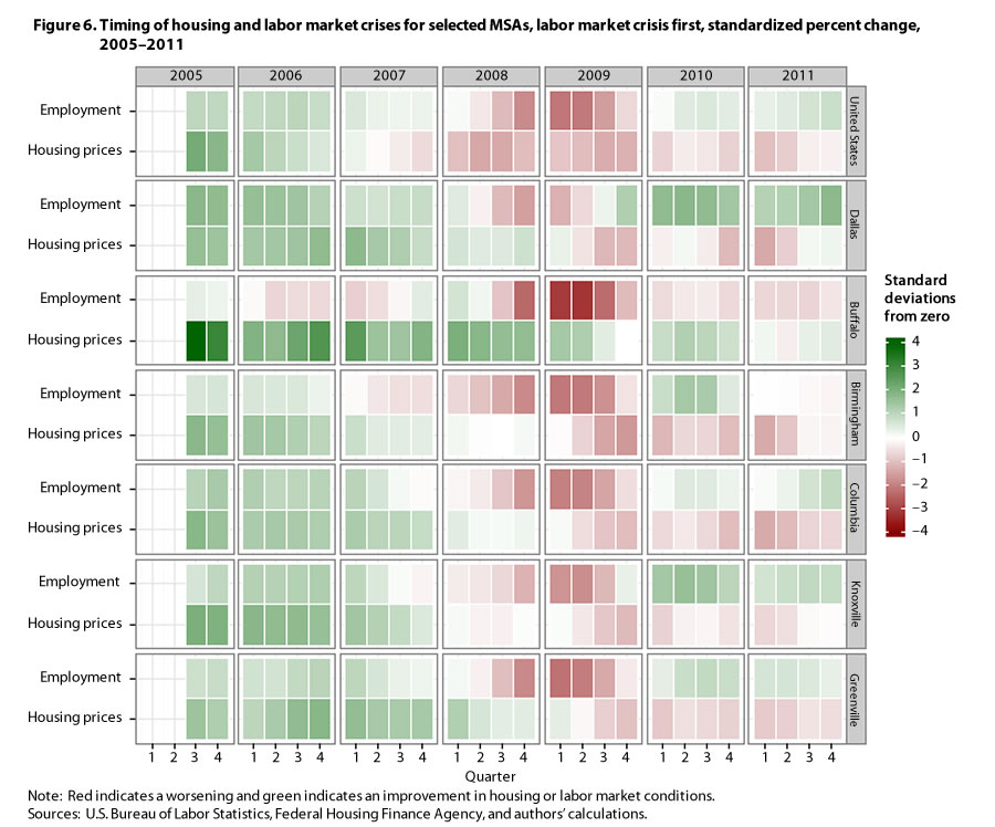
| MSA ID | City | Date | Variable | Standard deviations from zero |
|---|---|---|---|---|
0 | United States | August 15, 2005 | Employment | 1.02 |
13820 | Birmingham | August 15, 2005 | Employment | .63 |
15380 | Buffalo | August 15, 2005 | Employment | .41 |
17900 | Columbia | August 15, 2005 | Employment | 1.10 |
19124 | Dallas | August 15, 2005 | Employment | 1.81 |
24860 | Greenville | August 15, 2005 | Employment | .80 |
28940 | Knoxville | August 15, 2005 | Employment | .66 |
0 | United States | November 15, 2005 | Employment | .99 |
13820 | Birmingham | November 15, 2005 | Employment | .64 |
15380 | Buffalo | November 15, 2005 | Employment | .27 |
17900 | Columbia | November 15, 2005 | Employment | 1.34 |
19124 | Dallas | November 15, 2005 | Employment | 1.74 |
24860 | Greenville | November 15, 2005 | Employment | .86 |
28940 | Knoxville | November 15, 2005 | Employment | 1.02 |
0 | United States | February 14, 2006 | Employment | .93 |
13820 | Birmingham | February 14, 2006 | Employment | .62 |
15380 | Buffalo | February 14, 2006 | Employment | –.08 |
17900 | Columbia | February 14, 2006 | Employment | 1.24 |
19124 | Dallas | February 14, 2006 | Employment | 1.64 |
24860 | Greenville | February 14, 2006 | Employment | .74 |
28940 | Knoxville | February 14, 2006 | Employment | 1.18 |
0 | United States | May 16, 2006 | Employment | 1.00 |
13820 | Birmingham | May 16, 2006 | Employment | .60 |
15380 | Buffalo | May 16, 2006 | Employment | –.66 |
17900 | Columbia | May 16, 2006 | Employment | 1.02 |
19124 | Dallas | May 16, 2006 | Employment | 1.56 |
24860 | Greenville | May 16, 2006 | Employment | .71 |
28940 | Knoxville | May 16, 2006 | Employment | 1.13 |
0 | United States | August 15, 2006 | Employment | 1.06 |
13820 | Birmingham | August 15, 2006 | Employment | .59 |
15380 | Buffalo | August 15, 2006 | Employment | –.56 |
17900 | Columbia | August 15, 2006 | Employment | 1.04 |
19124 | Dallas | August 15, 2006 | Employment | 1.51 |
24860 | Greenville | August 15, 2006 | Employment | .94 |
28940 | Knoxville | August 15, 2006 | Employment | 1.19 |
0 | United States | November 15, 2006 | Employment | .87 |
13820 | Birmingham | November 15, 2006 | Employment | .30 |
15380 | Buffalo | November 15, 2006 | Employment | –.60 |
17900 | Columbia | November 15, 2006 | Employment | 1.12 |
19124 | Dallas | November 15, 2006 | Employment | 1.15 |
24860 | Greenville | November 15, 2006 | Employment | 1.10 |
28940 | Knoxville | November 15, 2006 | Employment | 1.26 |
0 | United States | February 14, 2007 | Employment | .59 |
13820 | Birmingham | February 14, 2007 | Employment | –.08 |
15380 | Buffalo | February 14, 2007 | Employment | –.76 |
17900 | Columbia | February 14, 2007 | Employment | 1.10 |
19124 | Dallas | February 14, 2007 | Employment | .81 |
24860 | Greenville | February 14, 2007 | Employment | 1.03 |
28940 | Knoxville | February 14, 2007 | Employment | 1.03 |
0 | United States | May 16, 2007 | Employment | .32 |
13820 | Birmingham | May 16, 2007 | Employment | –.39 |
15380 | Buffalo | May 16, 2007 | Employment | –.51 |
17900 | Columbia | May 16, 2007 | Employment | .66 |
19124 | Dallas | May 16, 2007 | Employment | .71 |
24860 | Greenville | May 16, 2007 | Employment | .64 |
28940 | Knoxville | May 16, 2007 | Employment | .58 |
0 | United States | August 15, 2007 | Employment | .26 |
13820 | Birmingham | August 15, 2007 | Employment | –.50 |
15380 | Buffalo | August 15, 2007 | Employment | –.12 |
17900 | Columbia | August 15, 2007 | Employment | .15 |
19124 | Dallas | August 15, 2007 | Employment | .85 |
24860 | Greenville | August 15, 2007 | Employment | .34 |
28940 | Knoxville | August 15, 2007 | Employment | .10 |
0 | United States | November 15, 2007 | Employment | .29 |
13820 | Birmingham | November 15, 2007 | Employment | –.51 |
15380 | Buffalo | November 15, 2007 | Employment | .46 |
17900 | Columbia | November 15, 2007 | Employment | –.06 |
19124 | Dallas | November 15, 2007 | Employment | .89 |
24860 | Greenville | November 15, 2007 | Employment | .26 |
28940 | Knoxville | November 15, 2007 | Employment | –.18 |
0 | United States | February 15, 2008 | Employment | .11 |
13820 | Birmingham | February 15, 2008 | Employment | –.63 |
15380 | Buffalo | February 15, 2008 | Employment | .69 |
17900 | Columbia | February 15, 2008 | Employment | –.14 |
19124 | Dallas | February 15, 2008 | Employment | .51 |
24860 | Greenville | February 15, 2008 | Employment | .16 |
28940 | Knoxville | February 15, 2008 | Employment | –.31 |
0 | United States | May 16, 2008 | Employment | –.37 |
13820 | Birmingham | May 16, 2008 | Employment | –.94 |
15380 | Buffalo | May 16, 2008 | Employment | .21 |
17900 | Columbia | May 16, 2008 | Employment | –.33 |
19124 | Dallas | May 16, 2008 | Employment | –.22 |
24860 | Greenville | May 16, 2008 | Employment | –.23 |
28940 | Knoxville | May 16, 2008 | Employment | –.38 |
0 | United States | August 15, 2008 | Employment | –1.09 |
13820 | Birmingham | August 15, 2008 | Employment | –1.35 |
15380 | Buffalo | August 15, 2008 | Employment | –.93 |
17900 | Columbia | August 15, 2008 | Employment | –.89 |
19124 | Dallas | August 15, 2008 | Employment | –1.08 |
24860 | Greenville | August 15, 2008 | Employment | –1.01 |
28940 | Knoxville | August 15, 2008 | Employment | –.63 |
0 | United States | November 15, 2008 | Employment | –1.82 |
13820 | Birmingham | November 15, 2008 | Employment | –1.83 |
15380 | Buffalo | November 15, 2008 | Employment | –2.36 |
17900 | Columbia | November 15, 2008 | Employment | –1.63 |
19124 | Dallas | November 15, 2008 | Employment | –1.49 |
24860 | Greenville | November 15, 2008 | Employment | –1.86 |
28940 | Knoxville | November 15, 2008 | Employment | –1.20 |
0 | United States | February 14, 2009 | Employment | –2.15 |
13820 | Birmingham | February 14, 2009 | Employment | –2.13 |
15380 | Buffalo | February 14, 2009 | Employment | –3.11 |
17900 | Columbia | February 14, 2009 | Employment | –2.00 |
19124 | Dallas | February 14, 2009 | Employment | –1.22 |
24860 | Greenville | February 14, 2009 | Employment | –2.22 |
28940 | Knoxville | February 14, 2009 | Employment | –1.69 |
0 | United States | May 16, 2009 | Employment | –2.10 |
13820 | Birmingham | May 16, 2009 | Employment | –2.11 |
15380 | Buffalo | May 16, 2009 | Employment | –3.19 |
17900 | Columbia | May 16, 2009 | Employment | –1.95 |
19124 | Dallas | May 16, 2009 | Employment | –.60 |
24860 | Greenville | May 16, 2009 | Employment | –2.04 |
28940 | Knoxville | May 16, 2009 | Employment | –1.77 |
0 | United States | August 15, 2009 | Employment | –1.54 |
13820 | Birmingham | August 15, 2009 | Employment | –1.72 |
15380 | Buffalo | August 15, 2009 | Employment | –2.32 |
17900 | Columbia | August 15, 2009 | Employment | –1.42 |
19124 | Dallas | August 15, 2009 | Employment | .27 |
24860 | Greenville | August 15, 2009 | Employment | –1.34 |
28940 | Knoxville | August 15, 2009 | Employment | –1.12 |
0 | United States | November 15, 2009 | Employment | –.61 |
13820 | Birmingham | November 15, 2009 | Employment | –.45 |
15380 | Buffalo | November 15, 2009 | Employment | –1.06 |
17900 | Columbia | November 15, 2009 | Employment | –.52 |
19124 | Dallas | November 15, 2009 | Employment | 1.23 |
24860 | Greenville | November 15, 2009 | Employment | –.34 |
28940 | Knoxville | November 15, 2009 | Employment | .35 |
0 | United States | February 14, 2010 | Employment | .09 |
13820 | Birmingham | February 14, 2010 | Employment | .84 |
15380 | Buffalo | February 14, 2010 | Employment | –.57 |
17900 | Columbia | February 14, 2010 | Employment | .13 |
19124 | Dallas | February 14, 2010 | Employment | 1.72 |
24860 | Greenville | February 14, 2010 | Employment | .42 |
28940 | Knoxville | February 14, 2010 | Employment | 1.43 |
0 | United States | May 16, 2010 | Employment | .50 |
13820 | Birmingham | May 16, 2010 | Employment | 1.41 |
15380 | Buffalo | May 16, 2010 | Employment | –.35 |
17900 | Columbia | May 16, 2010 | Employment | .53 |
19124 | Dallas | May 16, 2010 | Employment | 1.84 |
24860 | Greenville | May 16, 2010 | Employment | .84 |
28940 | Knoxville | May 16, 2010 | Employment | 1.62 |
0 | United States | August 15, 2010 | Employment | .57 |
13820 | Birmingham | August 15, 2010 | Employment | 1.34 |
15380 | Buffalo | August 15, 2010 | Employment | –.33 |
17900 | Columbia | August 15, 2010 | Employment | .52 |
19124 | Dallas | August 15, 2010 | Employment | 1.72 |
24860 | Greenville | August 15, 2010 | Employment | .96 |
28940 | Knoxville | August 15, 2010 | Employment | 1.49 |
0 | United States | November 15, 2010 | Employment | .46 |
13820 | Birmingham | November 15, 2010 | Employment | .53 |
15380 | Buffalo | November 15, 2010 | Employment | –.59 |
17900 | Columbia | November 15, 2010 | Employment | .29 |
19124 | Dallas | November 15, 2010 | Employment | 1.45 |
24860 | Greenville | November 15, 2010 | Employment | .85 |
28940 | Knoxville | November 15, 2010 | Employment | 1.08 |
0 | United States | February 14, 2011 | Employment | .39 |
13820 | Birmingham | February 14, 2011 | Employment | .02 |
15380 | Buffalo | February 14, 2011 | Employment | –.65 |
17900 | Columbia | February 14, 2011 | Employment | .10 |
19124 | Dallas | February 14, 2011 | Employment | 1.16 |
24860 | Greenville | February 14, 2011 | Employment | .66 |
28940 | Knoxville | February 14, 2011 | Employment | .72 |
0 | United States | May 16, 2011 | Employment | .51 |
13820 | Birmingham | May 16, 2011 | Employment | –.01 |
15380 | Buffalo | May 16, 2011 | Employment | –.63 |
17900 | Columbia | May 16, 2011 | Employment | .30 |
19124 | Dallas | May 16, 2011 | Employment | 1.18 |
24860 | Greenville | May 16, 2011 | Employment | .66 |
28940 | Knoxville | May 16, 2011 | Employment | .85 |
0 | United States | August 15, 2011 | Employment | .70 |
13820 | Birmingham | August 15, 2011 | Employment | –.10 |
15380 | Buffalo | August 15, 2011 | Employment | –.68 |
17900 | Columbia | August 15, 2011 | Employment | .71 |
19124 | Dallas | August 15, 2011 | Employment | 1.44 |
24860 | Greenville | August 15, 2011 | Employment | .56 |
28940 | Knoxville | August 15, 2011 | Employment | .96 |
0 | United States | November 15, 2011 | Employment | .82 |
13820 | Birmingham | November 15, 2011 | Employment | –.16 |
15380 | Buffalo | November 15, 2011 | Employment | –.40 |
17900 | Columbia | November 15, 2011 | Employment | .95 |
19124 | Dallas | November 15, 2011 | Employment | 1.79 |
24860 | Greenville | November 15, 2011 | Employment | .37 |
28940 | Knoxville | November 15, 2011 | Employment | .90 |
0 | United States | August 15, 2005 | Housing prices | 2.17 |
13820 | Birmingham | August 15, 2005 | Housing prices | 1.82 |
15380 | Buffalo | August 15, 2005 | Housing prices | 4.02 |
17900 | Columbia | August 15, 2005 | Housing prices | 1.86 |
19124 | Dallas | August 15, 2005 | Housing prices | 1.64 |
24860 | Greenville | August 15, 2005 | Housing prices | 1.53 |
28940 | Knoxville | August 15, 2005 | Housing prices | 2.07 |
0 | United States | November 15, 2005 | Housing prices | 1.85 |
13820 | Birmingham | November 15, 2005 | Housing prices | 1.66 |
15380 | Buffalo | November 15, 2005 | Housing prices | 3.15 |
17900 | Columbia | November 15, 2005 | Housing prices | 1.58 |
19124 | Dallas | November 15, 2005 | Housing prices | 1.54 |
24860 | Greenville | November 15, 2005 | Housing prices | 1.26 |
28940 | Knoxville | November 15, 2005 | Housing prices | 2.00 |
0 | United States | February 14, 2006 | Housing prices | 1.41 |
13820 | Birmingham | February 14, 2006 | Housing prices | 1.49 |
15380 | Buffalo | February 14, 2006 | Housing prices | 1.96 |
17900 | Columbia | February 14, 2006 | Housing prices | 1.32 |
19124 | Dallas | February 14, 2006 | Housing prices | 1.43 |
24860 | Greenville | February 14, 2006 | Housing prices | 1.05 |
28940 | Knoxville | February 14, 2006 | Housing prices | 1.85 |
0 | United States | May 16, 2006 | Housing prices | 1.06 |
13820 | Birmingham | May 16, 2006 | Housing prices | 1.41 |
15380 | Buffalo | May 16, 2006 | Housing prices | 1.77 |
17900 | Columbia | May 16, 2006 | Housing prices | 1.38 |
19124 | Dallas | May 16, 2006 | Housing prices | 1.45 |
24860 | Greenville | May 16, 2006 | Housing prices | 1.34 |
28940 | Knoxville | May 16, 2006 | Housing prices | 1.74 |
0 | United States | August 15, 2006 | Housing prices | .82 |
13820 | Birmingham | August 15, 2006 | Housing prices | 1.22 |
15380 | Buffalo | August 15, 2006 | Housing prices | 2.31 |
17900 | Columbia | August 15, 2006 | Housing prices | 1.33 |
19124 | Dallas | August 15, 2006 | Housing prices | 1.52 |
24860 | Greenville | August 15, 2006 | Housing prices | 1.71 |
28940 | Knoxville | August 15, 2006 | Housing prices | 1.76 |
0 | United States | November 15, 2006 | Housing prices | .61 |
13820 | Birmingham | November 15, 2006 | Housing prices | 1.07 |
15380 | Buffalo | November 15, 2006 | Housing prices | 2.73 |
17900 | Columbia | November 15, 2006 | Housing prices | 1.28 |
19124 | Dallas | November 15, 2006 | Housing prices | 1.73 |
24860 | Greenville | November 15, 2006 | Housing prices | 1.87 |
28940 | Knoxville | November 15, 2006 | Housing prices | 1.61 |
0 | United States | February 14, 2007 | Housing prices | .31 |
13820 | Birmingham | February 14, 2007 | Housing prices | .82 |
15380 | Buffalo | February 14, 2007 | Housing prices | 2.59 |
17900 | Columbia | February 14, 2007 | Housing prices | 1.32 |
19124 | Dallas | February 14, 2007 | Housing prices | 1.79 |
24860 | Greenville | February 14, 2007 | Housing prices | 1.68 |
28940 | Knoxville | February 14, 2007 | Housing prices | 1.47 |
0 | United States | May 16, 2007 | Housing prices | –.06 |
13820 | Birmingham | May 16, 2007 | Housing prices | .49 |
15380 | Buffalo | May 16, 2007 | Housing prices | 1.55 |
17900 | Columbia | May 16, 2007 | Housing prices | 1.08 |
19124 | Dallas | May 16, 2007 | Housing prices | 1.39 |
24860 | Greenville | May 16, 2007 | Housing prices | 1.38 |
28940 | Knoxville | May 16, 2007 | Housing prices | 1.17 |
0 | United States | August 15, 2007 | Housing prices | –.30 |
13820 | Birmingham | August 15, 2007 | Housing prices | .47 |
15380 | Buffalo | August 15, 2007 | Housing prices | 1.51 |
17900 | Columbia | August 15, 2007 | Housing prices | 1.08 |
19124 | Dallas | August 15, 2007 | Housing prices | 1.26 |
24860 | Greenville | August 15, 2007 | Housing prices | 1.33 |
28940 | Knoxville | August 15, 2007 | Housing prices | .93 |
0 | United States | November 15, 2007 | Housing prices | –.57 |
13820 | Birmingham | November 15, 2007 | Housing prices | .44 |
15380 | Buffalo | November 15, 2007 | Housing prices | 1.92 |
17900 | Columbia | November 15, 2007 | Housing prices | .90 |
19124 | Dallas | November 15, 2007 | Housing prices | .89 |
24860 | Greenville | November 15, 2007 | Housing prices | 1.40 |
28940 | Knoxville | November 15, 2007 | Housing prices | .56 |
0 | United States | February 15, 2008 | Housing prices | –.99 |
13820 | Birmingham | February 15, 2008 | Housing prices | .19 |
15380 | Buffalo | February 15, 2008 | Housing prices | 2.07 |
17900 | Columbia | February 15, 2008 | Housing prices | .47 |
19124 | Dallas | February 15, 2008 | Housing prices | .67 |
24860 | Greenville | February 15, 2008 | Housing prices | 1.22 |
28940 | Knoxville | February 15, 2008 | Housing prices | .13 |
0 | United States | May 16, 2008 | Housing prices | –1.38 |
13820 | Birmingham | May 16, 2008 | Housing prices | –.01 |
15380 | Buffalo | May 16, 2008 | Housing prices | 1.87 |
17900 | Columbia | May 16, 2008 | Housing prices | .15 |
19124 | Dallas | May 16, 2008 | Housing prices | .51 |
24860 | Greenville | May 16, 2008 | Housing prices | .64 |
28940 | Knoxville | May 16, 2008 | Housing prices | –.19 |
0 | United States | August 15, 2008 | Housing prices | –1.35 |
13820 | Birmingham | August 15, 2008 | Housing prices | –.01 |
15380 | Buffalo | August 15, 2008 | Housing prices | 1.69 |
17900 | Columbia | August 15, 2008 | Housing prices | .13 |
19124 | Dallas | August 15, 2008 | Housing prices | .54 |
24860 | Greenville | August 15, 2008 | Housing prices | .43 |
28940 | Knoxville | August 15, 2008 | Housing prices | –.22 |
0 | United States | November 15, 2008 | Housing prices | –1.02 |
13820 | Birmingham | November 15, 2008 | Housing prices | .15 |
15380 | Buffalo | November 15, 2008 | Housing prices | 1.71 |
17900 | Columbia | November 15, 2008 | Housing prices | .26 |
19124 | Dallas | November 15, 2008 | Housing prices | .77 |
24860 | Greenville | November 15, 2008 | Housing prices | .46 |
28940 | Knoxville | November 15, 2008 | Housing prices | .04 |
0 | United States | February 14, 2009 | Housing prices | –.90 |
13820 | Birmingham | February 14, 2009 | Housing prices | –.05 |
15380 | Buffalo | February 14, 2009 | Housing prices | 1.42 |
17900 | Columbia | February 14, 2009 | Housing prices | .11 |
19124 | Dallas | February 14, 2009 | Housing prices | .34 |
24860 | Greenville | February 14, 2009 | Housing prices | .41 |
28940 | Knoxville | February 14, 2009 | Housing prices | .06 |
0 | United States | May 16, 2009 | Housing prices | –1.02 |
13820 | Birmingham | May 16, 2009 | Housing prices | –.70 |
15380 | Buffalo | May 16, 2009 | Housing prices | 1.27 |
17900 | Columbia | May 16, 2009 | Housing prices | –.55 |
19124 | Dallas | May 16, 2009 | Housing prices | –.44 |
24860 | Greenville | May 16, 2009 | Housing prices | –.11 |
28940 | Knoxville | May 16, 2009 | Housing prices | –.37 |
0 | United States | August 15, 2009 | Housing prices | –1.29 |
13820 | Birmingham | August 15, 2009 | Housing prices | –1.41 |
15380 | Buffalo | August 15, 2009 | Housing prices | .46 |
17900 | Columbia | August 15, 2009 | Housing prices | –.91 |
19124 | Dallas | August 15, 2009 | Housing prices | –1.12 |
24860 | Greenville | August 15, 2009 | Housing prices | –.76 |
28940 | Knoxville | August 15, 2009 | Housing prices | –.88 |
0 | United States | November 15, 2009 | Housing prices | –1.23 |
13820 | Birmingham | November 15, 2009 | Housing prices | –1.61 |
15380 | Buffalo | November 15, 2009 | Housing prices | .00 |
17900 | Columbia | November 15, 2009 | Housing prices | –1.03 |
19124 | Dallas | November 15, 2009 | Housing prices | –1.10 |
24860 | Greenville | November 15, 2009 | Housing prices | –.96 |
28940 | Knoxville | November 15, 2009 | Housing prices | –1.08 |
0 | United States | February 14, 2010 | Housing prices | –.69 |
13820 | Birmingham | February 14, 2010 | Housing prices | –1.11 |
15380 | Buffalo | February 14, 2010 | Housing prices | .87 |
17900 | Columbia | February 14, 2010 | Housing prices | –.60 |
19124 | Dallas | February 14, 2010 | Housing prices | –.26 |
24860 | Greenville | February 14, 2010 | Housing prices | –.86 |
28940 | Knoxville | February 14, 2010 | Housing prices | –.71 |
0 | United States | May 16, 2010 | Housing prices | –.30 |
13820 | Birmingham | May 16, 2010 | Housing prices | –.63 |
15380 | Buffalo | May 16, 2010 | Housing prices | 1.22 |
17900 | Columbia | May 16, 2010 | Housing prices | –.35 |
19124 | Dallas | May 16, 2010 | Housing prices | .17 |
24860 | Greenville | May 16, 2010 | Housing prices | –.50 |
28940 | Knoxville | May 16, 2010 | Housing prices | –.20 |
0 | United States | August 15, 2010 | Housing prices | –.38 |
13820 | Birmingham | August 15, 2010 | Housing prices | –.66 |
15380 | Buffalo | August 15, 2010 | Housing prices | 1.07 |
17900 | Columbia | August 15, 2010 | Housing prices | –.62 |
19124 | Dallas | August 15, 2010 | Housing prices | –.29 |
24860 | Greenville | August 15, 2010 | Housing prices | –.62 |
28940 | Knoxville | August 15, 2010 | Housing prices | –.16 |
0 | United States | November 15, 2010 | Housing prices | –.72 |
13820 | Birmingham | November 15, 2010 | Housing prices | –1.04 |
15380 | Buffalo | November 15, 2010 | Housing prices | .80 |
17900 | Columbia | November 15, 2010 | Housing prices | –1.03 |
19124 | Dallas | November 15, 2010 | Housing prices | –1.07 |
24860 | Greenville | November 15, 2010 | Housing prices | –.73 |
28940 | Knoxville | November 15, 2010 | Housing prices | –.43 |
0 | United States | February 14, 2011 | Housing prices | –.97 |
13820 | Birmingham | February 14, 2011 | Housing prices | –1.32 |
15380 | Buffalo | February 14, 2011 | Housing prices | .23 |
17900 | Columbia | February 14, 2011 | Housing prices | –1.31 |
19124 | Dallas | February 14, 2011 | Housing prices | –1.35 |
24860 | Greenville | February 14, 2011 | Housing prices | –.82 |
28940 | Knoxville | February 14, 2011 | Housing prices | –.65 |
0 | United States | May 16, 2011 | Housing prices | –.78 |
13820 | Birmingham | May 16, 2011 | Housing prices | –.88 |
15380 | Buffalo | May 16, 2011 | Housing prices | –.27 |
17900 | Columbia | May 16, 2011 | Housing prices | –1.06 |
19124 | Dallas | May 16, 2011 | Housing prices | –.78 |
24860 | Greenville | May 16, 2011 | Housing prices | –.76 |
28940 | Knoxville | May 16, 2011 | Housing prices | –.50 |
0 | United States | August 15, 2011 | Housing prices | –.25 |
13820 | Birmingham | August 15, 2011 | Housing prices | –.15 |
15380 | Buffalo | August 15, 2011 | Housing prices | .38 |
17900 | Columbia | August 15, 2011 | Housing prices | –.68 |
19124 | Dallas | August 15, 2011 | Housing prices | .18 |
24860 | Greenville | August 15, 2011 | Housing prices | –.44 |
28940 | Knoxville | August 15, 2011 | Housing prices | –.08 |
0 | United States | November 15, 2011 | Housing prices | –.23 |
13820 | Birmingham | November 15, 2011 | Housing prices | –.18 |
15380 | Buffalo | November 15, 2011 | Housing prices | .49 |
17900 | Columbia | November 15, 2011 | Housing prices | –.64 |
19124 | Dallas | November 15, 2011 | Housing prices | .25 |
24860 | Greenville | November 15, 2011 | Housing prices | –.54 |
28940 | Knoxville | November 15, 2011 | Housing prices | –.05 |
Sources: U.S. Bureau of Labor Statistics, Federal Housing Finance Agency, and authors’ calculations. | ||||
Figures 5 and 6 use quarterly data for the period 2005–2011 to highlight the timing, length, and severity of the housing and labor market crises for the 12 selected MSAs. The severity of the housing market crisis is measured by the percent change in housing prices, and the severity of the labor market crisis is measured by the percent change in employment. Because these series are measured in different units (housing price is an index and employment in MSA-level data is measured in thousands of people), the percent change reported for each series in figures 5 and 6 is standardized as follows:
%ΔXit / σxi ,
where %ΔXit is the annualized percent change in employment (or housing prices) for the ith MSA in quarter t, and σxi is the standard deviation of %ΔX within the ith MSA for the period 2005–2011.
As one example of the standardization procedure, consider the cell for employment in New York in third quarter 2005 in figure 5. The value reported in this cell is 1.35 standard deviations from 0 and was constructed as 2.08 percent (annualized value of percent change in quarterly employment in third quarter 2005 for New York) divided by 1.54 percent (standard deviation calculated across all quarters for New York for the period 2005–2011). For further ease of interpretation of figures 5 and 6, darker colors indicate a larger number of standard deviations in the measure from zero, with red indicating a worsening and green indicating an improvement in housing or labor market conditions. Both figures also include the United States (all 353 MSAs aggregated) in the top panel for comparison purposes.
Figure 5 focuses on the experience of the six selected “housing crisis first” MSAs. The timing of the crises can be seen by observing that the housing price series turns from green to red earlier (at least four quarters earlier, as specified) than does the employment series. Nonetheless, even among these six MSAs, there is still considerable variation. Las Vegas and San Diego experienced similar timing and relative magnitudes of change in housing prices and employment. Both saw housing prices peak well before employment peaked, and their housing price declines were relatively stronger compared with the eventual employment declines. Further, employment in Las Vegas had not picked up by 2011,41 and, as seen in figure 5, none of these six housing markets looked strong in 2011. By contrast, the situation in Washington, DC was considerably better, especially for the labor market, most likely because of the substantial number of public sector jobs which tend to be more recession proof.
Figure 6 points to the six selected “labor market crisis first” MSAs. The housing and labor market crises in these MSAs were generally far less severe in length and magnitude. In fact, the Dallas MSA was virtually unscathed, especially compared with the other large MSAs identified in figure 5. Buffalo is a notable exception and experienced a particularly deep labor market downturn from mid-2008 through late 2009; however, its housing market was little affected.42
The lower two panels of table 2 (which was introduced earlier) provide annual data for 2007 and 2010 on housing prices, employment, and other measures for the full set of “housing crisis first” and “labor market crisis first” MSAs. On average, employment fell by a similar percentage (about 5 percent) in both types of MSAs between 2007 and 2010, while housing prices declined by 32 percent in “housing crisis first” MSAs but experienced almost no change in “labor market crisis first” MSAs. Table 2 also provides supplementary information on foreclosure rates. As would be expected given the differential trends in housing prices, foreclosure rates rose considerably more in “housing crisis first” MSAs.
Trends in household formation. The final part of the analysis examines the association between the housing and labor market crises and household formation and homeownership by MSA. Table 4 presents pairwise correlations of all the variables (measured as year-to-year percent change) for all 353 MSAs and for the two types of MSAs. The correlation between changes in housing prices and changes in foreclosure rates is negative as expected (falling housing prices go hand in hand with rising foreclosure rates) and considerably stronger in “housing crisis first” MSAs (–0.71) than in “labor market crisis first” MSAs (–0.24). Another fairly strong association identified in “housing crisis first” MSAs is between changes in housing prices and changes in homeownership rates. The correlation is 0.46, compared with 0.21 for all MSAs and 0.20 for MSAs where the labor market fell first. Surprisingly, however, associations between changes in employment and changes in doubling up and associations between changes in housing prices and changes in doubling up are comparatively very weak and quite often not in expected directions across all 353 MSAs and by MSA type.
| All 353 MSAs | |||||||
|---|---|---|---|---|---|---|---|
| Employment (thousands) | House Price Index (2005 = 100) | Foreclosure rate (percent) | Homeownership rate | Household size | Nonrelatives in family households (percent) | Unmarried households (percent) | |
| Employment (thousands) | 1.00 | … | … | … | … | … | … |
| House Price Index (2005 = 100) | .39 | 1.00 | … | … | … | … | … |
| Foreclosure rate (percent) | –.10 | –.71 | 1.00 | … | … | … | … |
| Homeownership rate (percent) | .00 | .21 | –.08 | 1.00 | … | … | … |
| Household size | .06 | –.07 | .22 | .12 | 1.00 | … | … |
| Nonrelatives in family households (percent) | .12 | .08 | –.05 | –.06 | –.06 | 1.00 | … |
| Unmarried households (percent) | .11 | .09 | –.09 | –.14 | –.11 | .48 | 1.00 |
| Housing crisis first MSAs (55 MSAs) | |||||||
| Employment (thousands) | House Price Index (2005 = 100) | Foreclosure rate (percent) | Homeownership rate | Household size | Nonrelatives in family households (percent) | Unmarried households (percent) | |
| Employment (thousands) | 1.00 | … | … | … | … | … | … |
| House Price Index (2005 = 100) | .31 | 1.00 | … | … | … | … | … |
| Foreclosure rate (percent) | –.23 | –.71 | 1.00 | … | … | … | … |
| Homeownership rate (percent) | .09 | .46 | –.13 | 1.00 | … | … | … |
| Household size | .06 | –.05 | .40 | .25 | 1.00 | … | … |
| Nonrelatives in family households (percent) | .15 | .22 | –.19 | .17 | .04 | 1.00 | … |
| Unmarried households (percent) | .01 | –.03 | .22 | –.02 | –.03 | .31 | 1.00 |
| Labor market crisis first MSAs (67 MSAs) | |||||||
| Employment (thousands) | House Price Index (2005 = 100) | Foreclosure rate (percent) | Homeownership rate | Household size | Nonrelatives in family households (percent) | Unmarried households (percent) | |
| Employment (thousands) | 1.00 | … | … | … | … | … | … |
| House Price Index (2005 = 100) | .50 | 1.00 | … | … | … | … | … |
| Foreclosure rate (percent) | –.16 | –.24 | 1.00 | … | … | … | … |
| Homeownership rate (percent) | .05 | .20 | .05 | 1.00 | … | … | … |
| Household size | .02 | –.09 | –.10 | .02 | 1.00 | … | … |
| Nonrelatives in family households (percent) | .02 | –.02 | –.19 | .17 | .04 | 1.00 | … |
| Unmarried households (percent) | –.02 | –.05 | –.05 | –.28 | .02 | .33 | 1.00 |
| Notes: Note: The correlations are calculated on the basis of year-to-year percent changes in the variables. Sources: U.S. Bureau of Labor Statistics, Federal Housing Finance Agency, CoreLogic, American Community Survey, and authors' calculations. | |||||||
One explanation for why correlations between the crises and household formation are so weak at the MSA level may be that the preceding analysis does not take into account the fact that, as seen earlier, the housing and labor market crises occurred at different points in time in each MSA. For instance, even among “housing crisis first” MSAs, some MSAs continued to experience rising housing prices through 2007, while others had already begun to experience price declines. So, a final important step in the analysis is to match the substantive period (recall that figure 1 could be subdivided into four substantive periods) and the date. Table 5 takes a case-study approach for two representative MSAs: Las Vegas (housing crisis first) and Dallas (labor market crisis first). Because household formation is also studied, annual data for the period 2005–2010 are used. These data are divided into three substantive periods of interest: (1) from 2005 to the first market’s peak, (2) from the first market’s peak to the second market’s peak, and (3) from the second market’s peak to 2010. (Recall that a peak defines the start of a crisis.) In the case of Las Vegas, these substantive periods translate into the following three time frames: (1) from 2005 to 2006 (where 2006 refers to the housing market peak), (2) from 2006 (housing market peak) to 2008 (labor market peak), and (3) from 2008 (labor market peak) to 2010. A similar type of decomposition is done for Dallas. Because these substantive periods cover different numbers of years, all figures are reported as an average annual percent change to enable comparisons.
| Las Vegas, NV, housing crisis first MSA | ||||
|---|---|---|---|---|
| Variable | Average annual percent change (by period) | Total percent change (2005–2010) | ||
| Period 1: 2005 to housing market peak (2005–2006) | Period 2: from peak to peak (2006–2008) | Period 3: labor market peak to 2010 (2008–2010) | ||
| Employment (thousands) | 4.09 | 1.66 | –2.72 | 0.36 |
| House Price Index | 7.82 | –14.69 | –18.98 | –12.43 |
| Foreclosure rate (percent) | 90.88 | 181.68 | 65.30 | 110.55 |
| Homeownership rate (percent) | 1.81 | –1.96 | –2.79 | –1.55 |
| Household size | –2.07 | 1.72 | 1.07 | .69 |
| Nonrelatives in family households (percent) | –5.29 | –3.42 | 6.11 | –.10 |
| Unmarried households (percent) | 5.49 | 1.72 | 5.32 | 3.90 |
| Dallas, TX, labor market crisis first MSA | ||||
| Variable | Average annual percent change (by period) | Total percent change (2005–2010) | ||
| Period 1: 2005 to labor market peak (2005–2008) | Period 2: from peak to peak (2008–2009) | Period 3: housing market peak to 2010 (2009–2010) | ||
| Employment (thousands) | 1.03 | –1.31 | 1.89 | 0.73 |
| House Price Index | 2.43 | .33 | –.98 | 1.32 |
| Foreclosure rate (percent) | 12.20 | 30.62 | 23.62 | 17.93 |
| Homeownership rate (percent) | .47 | –1.73 | –.81 | –.23 |
| Household size | .77 | .43 | –3.53 | –.17 |
| Nonrelatives in family households (percent) | .90 | 16.42 | –5.37 | 2.51 |
| Unmarried households (percent) | –5.39 | 17.84 | 3.40 | .63 |
| Notes: Note: Housing and labor market peaks are identified in figures 5 and 6 by quarter and then reassigned to the relevant calendar year. A peak is used to define the start of a crisis. Sources: U.S. Bureau of Labor Statistics, Federal Housing Finance Agency, CoreLogic, American Community Survey, and authors' calculations. | ||||
First consider the Las Vegas MSA. In period 1, employment and housing prices were rising at annual rates of 4 percent and nearly 8 percent, respectively. At the same time, homeownership was rising at an annual rate of nearly 2 percent, and both average household size and the percentage of nonrelatives living in family households were falling. Increases in the homeownership rate may reflect rising investment demand for housing, whereas declines in doubling up may reflect an increase in the consumption demand for housing. In period 2 (housing market crisis only), employment growth slowed compared with the previous period, while housing prices fell by 15 percent annually and the foreclosure rate rose dramatically.43 In this period, the homeownership rate fell by 2 percent annually and average household size rose by 1.7 percent annually. While the percentage of nonrelatives living in family households continued to fall (rather than rise, as might be expected), the percent decline in period 2 was, nonetheless, smaller than the decline in period 1. The percentage of unmarried households continued to rise, although, surprisingly, at a lower rate. Finally, in period 3, with both crises underway, employment fell by 2.7 percent annually and housing prices declined even more than they did in the previous period, falling by nearly 19 percent annually. And, as would be expected, the percentage of nonrelatives living in family households rose, as did the percentage of unmarried households. Household size also continued to increase, although not by as much as it did in period 2.
In Dallas, a “labor market crisis first” MSA, changes in housing conditions and employment were far more modest, consistent with figure 6 (which generally showed less severe crises for this MSA type). During period 2 (labor market crisis only), employment fell by just 1.3 percent annually, and there was only a modest decline in the homeownership rate (1.7 percent annually). Turning to changes in doubling up, there is no clear pattern; while household size was virtually unchanged, the percentage of nonrelatives living in family households increased considerably.44 In period 3, when the housing market declined, the fall in housing prices was slight (just 1 percent annually) and employment was growing again. The pickup in employment may explain concurrent declines in period 3, in both household size and the percentage of nonrelatives living in family households. Although this exercise suggests that isolating associations with the use of information on substantive timing is a potentially useful strategy for understanding housing decisions, it is important to keep in mind that these are just that—associations.
This article used data on 353 MSAs, with a focus on 12 MSAs, for the period from 2005 to 2011, to examine the relationship between the severity and relative timing of the housing and labor market crises and changes in household formation. Although it is well established that the U.S. housing market, as a whole, turned downward before the labor market did, this is the first study to look at the relative timing of these crises at the subnational level. The analysis showed that, contrary to the national pattern, in a slight majority of MSAs the labor market turned downward first.
MSAs where the housing market declined first have some distinct characteristics: (1) they are some of the largest areas (e.g., New York and Washington, DC) and are more often located on coasts; and (2) they experienced some of the most substantial downturns in the housing and labor markets, whether measured by the length of the crises, by the magnitude of the decline in housing prices or employment, or by the rise in foreclosures. Along with earlier work on the recent housing crisis,45 this article deepens our knowledge about the considerable heterogeneity in the experiences of MSAs, a phenomenon which is obscured when looking at the national picture or at just a handful of well-publicized MSAs.
The article also examined the association between changes in the housing and labor markets and changes in doubling up and homeownership. Declining housing prices were found to be strongly associated with declines in homeownership, especially in those MSAs where the housing crisis occurred before the labor market crisis. However, the association between changes in doubling up and the housing and labor market crises was found to be fairly weak at the MSA level. One explanation for this surprising finding is that the timing of the crises differed considerably across MSAs, necessitating more refined analyses. This study is just a first step in this direction. Factors, such as migration and age distribution of household heads, are not accounted for in the analysis, and finding association is not the same as establishing causation (which is not addressed or claimed here). A logical next step in this line of research is to take advantage of the observed heterogeneity in the experiences of MSAs—heterogeneity in terms of the severity, length, and timing of the recent housing and labor market crises, as identified here—and examine impacts on individual decisions regarding doubling up, homeownership, and cohabitation.
Table A–1 presents the data used in conjunction with information on housing and labor market peaks to make the computations used in table 5.
| Data for Las Vegas, NV, housing crisis first MSA | ||||||
|---|---|---|---|---|---|---|
| Variable | 2005 | 2006 | 2007 | 2008 | 2009 | 2010 |
| Employment (thousands) | 838.9 | 873.2 | 890.1 | 902.4 | 864.4 | 854.0 |
| House Price Index (2005 = 100) | 100.0 | 107.8 | 104.1 | 78.5 | 58.7 | 51.5 |
| Foreclosure rate (percent) | .22 | .41 | 1.36 | 3.28 | 6.61 | 8.97 |
| Homeownership rate (percent) | 59.47 | 60.55 | 58.62 | 58.20 | 56.88 | 54.99 |
| Household size | 3.63 | 3.55 | 3.58 | 3.67 | 3.66 | 3.75 |
| Nonrelatives in family households (percent) | 3.69 | 3.50 | 3.79 | 3.26 | 3.66 | 3.68 |
| Unmarried households (percent) | 8.94 | 9.43 | 10.21 | 9.76 | 10.28 | 10.83 |
| Data for Dallas, TX, labor market crisis first MSA | ||||||
| Variable | 2005 | 2006 | 2007 | 2008 | 2009 | 2010 |
| Employment (thousands) | 1,916.9 | 1,946.0 | 1,968.8 | 1,976.8 | 1,951.0 | 1,987.9 |
| House Price Index (2005 = 100) | 100.0 | 102.6 | 105.9 | 107.5 | 107.8 | 106.8 |
| Foreclosure rate (percent) | .65 | .65 | .73 | .91 | 1.19 | 1.47 |
| Homeownership rate (percent) | 61.05 | 62.08 | 62.66 | 61.91 | 60.84 | 60.34 |
| Household size | 3.78 | 3.84 | 3.85 | 3.87 | 3.89 | 3.75 |
| Nonrelatives in family households (percent) | 2.19 | 2.36 | 2.34 | 2.25 | 2.62 | 2.48 |
| Unmarried households (percent) | 7.32 | 6.57 | 6.28 | 6.20 | 7.31 | 7.55 |
| Notes: Sources: U.S. Bureau of Labor Statistics, Federal Housing Finance Agency, CoreLogic, American Community Survey, and authors' calculations. | ||||||
Acknowledgments: The authors gratefully acknowledge research funding from the University of Missouri Research Board. Trung Ly provided expert research assistance. The authors are grateful for comments from Deborah Balser, David Rose, Robert Sorensen, participants at the University of Missouri–St. Louis College of Business Seminar Series, and participants at the Washington University Seminar Series on Work, Family, and Policy.
!--?pagebreak>!--?pagebreak>!--?pagebreak>!--?pagebreak>!--?pagebreak>!--?pagebreak>!--?pagebreak>!--?pagebreak>!--?pagebreak>William H. Rogers, and Anne E. Winkler, "The relationship between the housing and labor market crises and doubling up: an MSA-level analysis, 2005–2011," Monthly Labor Review, U.S. Bureau of Labor Statistics, August 2013, https://doi.org/10.21916/mlr.2013.26
1 Christopher J. Goodman and Steven M. Mance, “Employment loss and the 2007–09 recession: an overview,” Monthly Labor Review, April 2011, pp. 3–12.
2 See Laryssa Mykyta and Suzanne Macartney, “The effects of recession on household composition: ‘doubling up’ and economic well-being,” SEHSD working paper 2011-4 (Washington, DC, U.S. Census Bureau, 2011), https://www.census.gov/hhes/www/poverty/publications/papers.html; Emily E. Wiemers, “The effect of unemployment on household composition and doubling up,” working paper (Boston, MA, University of Massachusetts–Boston, 2012); Pew Organization, “The return of the multi-generational family household,” Pew Research Social and Demographic Trends, 2010; and Dianna B. Elliott, Rebekah Young, and Jane L. Dye, “Variation in the formation of complex family households during the recession,” SEHSD working paper 2011-32 (Washington, DC, U.S. Census Bureau, 2011).
3 Even before the recent housing and labor market crises, demographers had noted the increasing rate of return (and delayed departure) of young adults from their parents’ homes. These trends were exacerbated by the depth and length of the recent housing and labor market crises; see Richard A. Settersten and Barbara Ray, “What’s going on with young people today? The long and twisting path to adulthood” Future of Children 20, Spring 2010, pp. 19–41.
4 Stephanie Armour, “More families move in together during housing crisis,” USA Today, February 3, 2009.
5 Rose Kreider, “Increase in opposite-sex cohabiting couples from 2009 to 2010 in the Annual Social and Economic Supplement (ASEC) to the Current Population Survey (CPS),” working paper (Washington, DC, U.S. Census Bureau, September 2010), https://www.census.gov/library/working-papers/2008/demo/kreider-02.html.
6 Previous examinations of timing at the subnational level largely focused on the housing market only. See Fernando Ferreira and Joseph Gyourko, “Anatomy of the beginning of the housing boom: U.S. neighborhoods and metropolitan areas, 1993–2009,” working paper 17374 (Cambridge, MA, National Bureau of Economic Research, 2011); and Todd M. Sinai, “House price moments in boom–bust cycles,” working paper 18059 (Cambridge, MA, National Bureau of Economic Research, May 2012). For a brief examination of the association between the crises and doubling up at the MSA level, see Timothy Dunne, “Household formation and the great recession,” Economic Commentary (Federal Reserve Bank of Cleveland, 2012).
7 See Kathryn J. Byun, “The U.S. housing bubble and bust: impacts on employment,” Monthly Labor Review, December 2010, pp. 3–17; and Jeffrey P. Cohen, Cletus C. Coughlin, and David A. Lopez, “The boom and bust of U.S. housing prices from various geographic perspectives,” Federal Reserve Bank of St. Louis Review 94, September/October 2012, pp. 341–367.
8 Cohen et al., “The boom and bust of U.S. housing prices.”
9 See Ibid.; and Sinai, “House price moments in boom–bust cycles.”
10 See Cohen et al., “The boom and bust of U.S. housing prices.”
11 See Karl E. Case and Robert J. Shiller, “Is there a bubble in the housing market?” Brookings Papers on Economic Activity 2, 2003, pp. 299–342, http://www.econ.yale.edu/~shiller/pubs/p1089.pdf; Ferreira and Gyourko, “Anatomy of the beginning of the housing boom;” and Sinai, “House price moments in boom–bust cycles.”
12 Sinai, “House price moments in boom–bust cycles.”
13 Robert Lerman and Thomas Kingsley, “Metro areas suffering the worst housing shocks also lose the most jobs,” Metro Trends (Washington, DC, Urban Institute, 2010).
14 Byun, “The U.S. housing bubble bust.”
15 Howard H. Wall, “The employment cycles of neighboring cities,” Regional Science and Urban Economics 43, no. 1, 2013, pp. 177–185.
16 In recent years, quite a few studies have identified a relationship between the advent of the Great Recession and doubling up at the national level. Before the recent crisis, a substantial body of social science research focused on the relationship between housing conditions and household formation decisions of individuals (principally young adults and single mothers). Such studies include Axel Borsch-Supan, “Household formation, housing prices, and public policy impacts,” Journal of Public Economics 30, July 1986, pp. 145–164; David Card and Thomas Lemieux, “Adapting to circumstances: the evolution of work, school, and living arrangements among North American youth,” in David Blanchflower and Richard Freeman, eds., Youth Employment and Joblessness in Advanced Countries (Chicago, University of Chicago Press, 1999); John F. Ermisch, “Prices, parents, and young people’s household formation,” Journal of Urban Economics 45, January 1999, pp. 47–71; Frank F. Furstenberg, “On a new schedule: transitions to adulthood and family change,” Future of Children 20, Spring 2010, pp. 67–87; Frances K. Goldscheider and Julie DaVanzo, “Pathways to independent living in early adulthood: marriage, semiautonomy, and premarital residential independence,” Demography 26, November 1989, pp. 597–614; Donald R. Haurin and Stuart Rosenthal, “The influence of household formation on homeownership rates across time and race,” Real Estate Economics 35, December 2007, pp. 411–450; Anne E. Winkler, “The impact of housing costs on the living arrangements of single mothers,” Journal of Urban Economics 32, November 1992, pp. 388–403; Aaron Yelowitz, “Young adults leaving the nest: the role of the cost of living,” in Sheldon Danziger and Cecilia Elena Rouse, eds., The price of independence: the economics of early adulthood (New York, Russell Sage, 2007), pp. 170–206; and Zhu X. Di and Xiaodong Liu, “The effects of housing push factors and rent expectations on household formation of young adults,” Journal of Real Estate Research 28, no. 2, 2006, pp. 149–166.
17 A headship rate is defined as the fraction of adults who are heads of households.
18 Dunne, “Household formation and the great recession.”
19 Gary Painter, “What happens to household formation in a recession?” special report (Research Institute for Housing America, April 2010), http://www.housingamerica.org/RIHA/RIHA/Publications/72429_9821_Research_RIHA_Household_Report.pdf.
20 Lisa J. Dettling and Melissa S. Kearney, “House prices and birth rates: the impact of the real estate market on the decision to have a baby,” working paper 17485 (Cambridge, MA, National Bureau of Economic Research, October 2011).
21 For example, see Atif R. Mian, Amir Sufi, and Francesco Trebbi, “Foreclosures, house prices, and the real economy,” working paper 16685 (Cambridge, MA, National Bureau of Economic Research, January 2011); William H. Rogers, “Declining foreclosure neighborhood effects over time,” Housing Policy Debate 20, September 2010, pp. 687–706; William H. Rogers and William Winter, “The impact of foreclosures on neighboring housing sales,” Journal of Real Estate Research 31, no. 4, 2009, pp. 455–479; and John P. Harding, Eric Rosenblatt, and Vincent W. Yao, “The contagion effect of foreclosed properties,” Journal of Urban Economics 66, 2009, pp. 164–178.
22 The FHFA House Price Index series includes a total of 367 MSAs (metropolitan, micropolitan, and metro divisions). For this article, the figure is slightly reduced to 353 because of data availability for selected years in two other databases: CoreLogic and the annual ACS.
23 The advantage of looking at employment rather than unemployment is that unemployed status depends on job-search activity. Only figure 1 provides information on both employment and the unemployment rate.
24 FHFA constant-quality housing prices are constructed using a repeat-sales method (similar to the Case-Shiller index), where sales observations are not included unless the housing unit has been sold at least twice in the data series. One characteristic of a repeat-sales index is that previously published values are subject to change over time, as existing housing units are sold a second time. The present analysis uses data collected from FHFA in the summer of 2012. Thus, the rates of change calculated here may not precisely match reported rates in current or future FHFA publications.
25 See Cohen et al., “The boom and bust of U.S. housing prices;” and Sinai, “House price moments in boom–bust cycles.”
26 For a comparison with other sources of foreclosure data, including RealtyTrac, see “Sources of foreclosure data,” MBA Research DataNotes (Mortgage Bankers Association, 2008), http://www.mortgagebankers.org/files/Research/July2008SourcesofForeclosureData.pdf. The report by the Mortgage Bankers Association points to an important drawback of the oft-used RealtyTrac measure: the measure is subject to double counting. Although RealtyTrac only counts one filing per month (even if more than one occurs), if filings for the same property occur in different months, RealtyTrac counts all such events.
27 Robert B. Cleveland, William S. Cleveland, Jean E. McRae, and Irma Terpenning, “STL: a seasonal-trend decomposition procedure based on loess,” Journal of Official Statistics 6, 1990, pp. 3–73.
28 The U.S. Census Bureau defines a family household as a household in which there is at least one person present who is related to the householder by birth, marriage, or adoption. (See U.S. Census Bureau website, https://www.census.gov/hhes/families/about/.)
29 Pamela Smock, Wendy Manning, and Meredith Porter, “‘Everything’s there except money:’ how money shapes decisions to marry among cohabitors,” Journal of Marriage and Family 67, August 2005, pp. 680–696.
30 Because the foreclosure data obtained by the authors from CoreLogic begin in second quarter 2005, all analyses use this period as the start date.
31 For a discussion of the unique set of events that precipitated the housing boom and the subsequent bust, see Karl E. Case and John M. Quigley, “How housing busts end: house prices, user cost and rigidities during down cycles,” in Susan J. Smith and Beverly A. Searle, eds., The Blackwell companion to the economics of housing: the housing wealth of nations (West Sussex, United Kingdom, Wiley–Blackwell, 2010). The authors describe the boom as being of “historical proportions.”
32 These figures were calculated by aggregating available monthly and quarterly data to the annual level.
33 As emphasized in this article, the timing of each crisis varied considerably by MSA, so the choice of 2007 is only for convenience of presentation.
34 Using weighted and unweighted MSAs, Sinai also points to a similar pattern of findings in his comparison of the severity of housing declines. (See Sinai, “House price moments in boom–bust cycles.”)
35 Kreider, “Increase in opposite-sex cohabiting couples.”
36 More precisely, a crisis is identified when the series growth rate from quarter to quarter changes sign, indicating a switch from growth to decline.
37 An alternative strategy is to identify the primary housing or labor market peak on the basis of the magnitude of the change in prices (or employment) rather than on the basis of duration. Most MSAs experienced multiple housing price peaks after the main downturn in their housing markets. However, because these housing price fluctuations were usually small in magnitude and duration, the first housing price downturn marked the peak of primary interest.
38 Besides MSAs excluded on the basis of the “four-quarter rule,” some additional MSAs were omitted from the set of “housing crisis first” and “labor market crisis first” MSAs to enable the subsequent annual analysis. Omitted MSAs also include those for which the period from peak to trough or from trough to peak could not be clearly identified. Clear identification of the period requires (1) one unit of time before the first peak in housing prices or employment, (2) one unit of time between peaks, and (3) one unit of time after the second peak in housing prices or employment. (A unit of time refers to a quarter or a year, depending on the analysis.) The omitted group includes a number of smaller MSAs and Boston. Boston, for example, saw housing prices peak in the summer of 2005 and employment peak in 2008. When the data for Boston were aggregated to annual rates of change to include household information, Boston no longer contained a prepeak period and was therefore dropped.
39 See Cohen et al., “The boom and bust of U.S. housing prices;” and Sinai, “House price moments in boom–bust cycles.”
40 Some notable cities are excluded from these lists. One exclusion already mentioned is Boston; another is Los Angeles. Although Los Angeles experienced the housing decline first, its labor market crisis occurred three quarters later, and so the city is not included based on the “four-quarter rule.”
41 In interpreting the magnitudes in figure 5, it is important to keep in mind the standardization that is used. The housing collapse in Las Vegas would stand out even more if the analysis had used the standard deviation of the percent change for all areas across the nation instead of the standard deviation of the percent change for the MSA itself. Standardizing each value by MSA allows one more quickly to identify strong changes in the employment and housing price growth within each MSA. This approach also permits meaningful comparisons of timing and magnitude across MSAs.
42 Buffalo is also notable in that it provides an example of the challenges in identifying peaks. Buffalo experienced two clear declines in employment: a small decline starting in 2006 and a larger decline starting in 2008. On the housing side, the decline in housing prices during the fourth quarter of 2009 is almost impossible to see, as growth returned in 2010. Further, in February 2013, FHFA reported a decline in housing prices in the first quarter of 2010 and not in 2009. This difference is due, in part, to an index calculation adjustment inherent in repeat-sales methods.
43 Although foreclosures increased considerably, the increase was due to a very low initial base.
44 It should be kept in mind that the sizeable increase is off of a very low base and that other factors are not held constant.
45 See Cohen et al., “The boom and bust of U.S. housing prices;” and Sinai, “House price moments in boom–bust cycles.”