
An official website of the United States government
An official website of the United States government
The .gov means it's official.
Federal government websites often end in .gov or .mil. Before sharing sensitive information,
make sure you're on a federal government site.
The site is secure.
The
https:// ensures that you are connecting to the official website and that any
information you provide is encrypted and transmitted securely.
February 2012
Architecture and engineering occupations are at the forefront of technological progress. Among the many possible tasks that workers in these jobs may perform are designing ships, aircraft, or computers; researching, developing, and evaluating medical devices; and devising improved processes for manufacturing products. Workers may use technical knowledge to design improved methods for extracting natural resources or to collect and analyze geographic information. Architecture and engineering jobs are highly skilled and high paying: nearly all of the occupations in this group pay above-average wages and typically require postsecondary education, often a bachelor’s degree or higher. This highlight provides an overview of employment and wages for architecture and engineering occupations, including information on industries in which architecture and engineering jobs are likely to be found and geographic areas in which these jobs are concentrated.
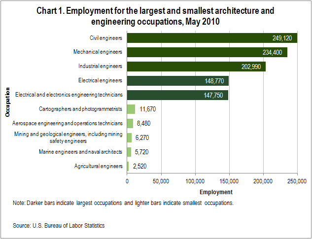
There were 2.3 million architecture and engineering jobs in 2010, representing about 2 percent of U.S. employment. By comparison, the two largest occupations, retail salespersons and cashiers, had employment of 4.2 and 3.4 million, respectively, more than all the architecture and engineering occupations combined. The largest architecture and engineering occupations were civil engineers, with employment of 249,120, mechanical engineers (234,400), and industrial engineers (202,900). Agricultural engineers (2,520), marine engineers and naval architects (5,720), and mining and geological engineers (6,270) were the smallest architecture and engineering occupations. (See chart 1.)
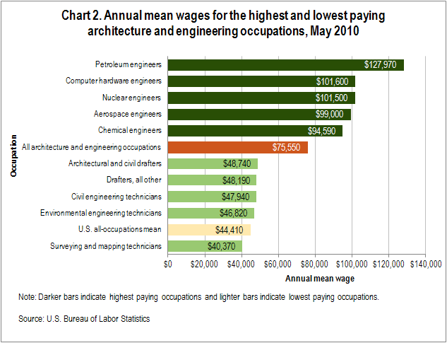
Although architecture and engineering was one of the smaller occupational groups, it was also one of the highest paying. The annual mean wage for the architecture and engineering group was $75,550, significantly above the U.S. all-occupations mean wage of $44,410 and exceeded only by the average wages for management ($105,440), legal ($96,940), and computer and mathematical ($77,230) occupations. Of the 35 architecture and engineering occupations, only one—surveying and mapping technicians—had a mean wage below the U.S. average. Among the highest paying architecture and engineering occupations were petroleum engineers ($127,970), computer hardware engineers ($101,600) and nuclear engineers ($101,500). Most of the lower paying architecture and engineering occupations were engineering technician or drafting jobs, which were typically held by workers with some college education or an associate’s degree. In addition to surveying and mapping technicians, with a mean annual wage of $40,370, the lowest paying architecture and engineering occupations included environmental engineering technicians ($46,820) and civil engineering technicians ($47,940). (See chart 2.)
Eighty-six percent of all architecture and engineering jobs were in the private sector and 14 percent were in the public sector, slightly below the public sector’s 17-percent employment share across all occupations. Private sector businesses that provided architectural, engineering, and related services were by far the largest employer of architecture and engineering occupations. Twenty-eight percent of all architecture and engineering jobs were found in the architectural, engineering, and related services industry, where these occupations represented half of total industry employment. Several high-tech manufacturing industries—aerospace product and parts manufacturing; navigational, measuring, electromedical, and control instruments manufacturing; and semiconductor and other electronic component manufacturing—also were among the largest employers of architecture and engineering occupations, each representing about 4 percent of total employment in this occupational group.
However, the distribution across industries varied for individual occupations within the architecture and engineering group. For example, more than 60 percent of petroleum engineers were employed in businesses that performed oil and gas extraction or support activities for mining, while industries employing the largest numbers of biomedical engineers included medical equipment and supplies manufacturing, scientific research and development services, and pharmaceutical and medicine manufacturing.
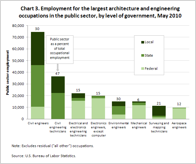
The share of public sector employment varied across individual architecture and engineering occupations, ranging from less than 1 percent of mechanical drafters and electrical and electronics drafters to about 47 percent of civil engineering technicians. Within the public sector, individual architecture and engineering occupations tended to be more prevalent at specific levels of government. Chart 3 shows employment for the largest architecture and engineering occupations in the public sector, broken down by level of government. The two engineering occupations with the highest public sector employment, civil engineers and civil engineering technicians, were primarily in state and local government. Both of these occupations also had relatively high shares of public sector employment overall. State government employed nearly half of public sector environmental engineers, and more than three-quarters of public sector surveying and mapping technicians were in local government. The federal government accounted for the majority of public sector employment in the remaining occupations shown, ranging from 71 percent of public sector electrical and electronics engineering technicians to 95 percent of public sector aerospace engineers.
The states with the highest employment and highest employment concentrations of selected engineering occupations are shown in Table 1. In general, states with high overall employment also tended to have the highest employment of most of the engineering occupations shown. Of the 18 engineering occupations listed in the table, California had the highest employment for 10 and Texas had the highest employment for 4; these were also the two states with the highest total employment of engineers.
| Occupation | State with highest location quotient | Location quotient in state with highest location quotient | Employment in state with highest location quotient | State with highest employment | Employment in state with highest employment | Location quotient in state with highest employment |
|---|---|---|---|---|---|---|
Aerospace engineers | Washington | 3.9 | 6,460 | California | 19,460 | 2.3 |
Agricultural engineers | North Dakota | 7.3 | 50 | Texas | 290 | 1.5 |
Biomedical engineers | Massachusetts | 3.9 | 1,440 | California | 3,820 | 2.3 |
Chemical engineers | Delaware | 7.9 | 710 | Texas | 5,030 | 2.2 |
Civil engineers | Alaska | 2.5 | 1,510 | California | 36,120 | 1.3 |
Computer hardware engineers | New Mexico | 3.8 | 1,570 | California | 17,780 | 2.4 |
Electrical engineers | Alaska | 2.3 | 810 | California | 18,320 | 1.1 |
Electronics engineers, except computer | Rhode Island | 2.3 | 1,080 | California | 27,170 | 1.8 |
Environmental engineers | Wyoming | 3.1 | 330 | California | 6,080 | 1.1 |
Health and safety engineers, except mining safety engineers and inspectors | Alaska | 2.6 | 150 | California | 2,360 | 0.9 |
Industrial engineers | Michigan | 3.3 | 19,680 | Michigan | 19,680 | 3.3 |
Marine engineers and naval architects | Virginia | 5.1 | 810 | Texas | 1,090 | 2.4 |
Materials engineers | Washington | 2.6 | 1,220 | California | 2,520 | 1.0 |
Mechanical engineers | Michigan | 4.4 | 30,260 | Michigan | 30,260 | 4.4 |
Mining and geological engineers, including mining safety engineers | Wyoming | 16.7 | 220 | Colorado | 680 | 6.4 |
Nuclear engineers | Tennessee | 4.0 | 1,520 | California | 3,180 | 1.6 |
Petroleum engineers | Alaska | 15.2 | 1,040 | Texas | 15,510 | 6.9 |
| Source: U.S. Bureau of Labor Statistics | ||||||
Although the architecture and engineering group made up about 1.8 percent of overall U.S. employment, its share of total employment varied by state from about 1 percent in Arkansas, South Dakota, and Nebraska to nearly 3 percent in Michigan, Alaska, and Washington. Employment shares of detailed architecture and engineering occupations varied more by state, as shown by the location quotient data in table 1. Location quotients are defined as the ratio of an occupation’s share of employment in a specific geographical area relative to its share of national employment; a location quotient greater than 1 indicates that the occupation makes up an above-average share of local employment. For example, an occupation that makes up 10 percent of local employment in a certain area, but only 2 percent of national employment, will have a location quotient of 5 in that area.
With the exception of industrial and mechanical engineers in Michigan, states with the highest employment of a given engineering occupation did not typically have the highest concentration of that occupation. For example, the employment share of health and safety engineers in Alaska was about 2.6 times the U.S. average, but this number represented only about 150 jobs. By comparison, the much larger state of California had nearly 16 times as many health and safety engineering jobs, despite a location quotient of only 0.9 for the occupation. In some cases, however, the state with the highest employment also had a high location quotient for that occupation. For example, Colorado had a location quotient of 6.4 for mining and geological engineers, and Texas had a location quotient of nearly 7 for petroleum engineers. However, these quotients were significantly lower than the location quotients for mining and geological engineers in Wyoming (16.7) and petroleum engineers in Alaska (15.2). These two location quotients were among the highest for any architecture and engineering occupation.
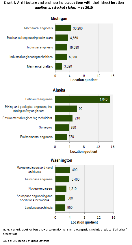
The architecture and engineering occupations with the highest location quotients in Michigan, Alaska, and Washington are shown in chart 4. Architecture and engineering occupations that made up an above-average share of employment in Michigan tended to be associated with manufacturing processes. Among these occupations were mechanical engineers and mechanical engineering technicians, industrial engineers and industrial engineering technicians, and mechanical drafters. The largest two were mechanical engineers and industrial engineers, with state employment of 30,260 and 19,680, respectively. Alaska had high concentrations of occupations associated with natural resource extraction; among these occupations were petroleum engineers, mining and geological engineers, environmental engineers, and occupations associated with geographical surveying and mapping, such as cartographers and photogrammetrists (not shown in the chart). Architecture and engineering occupations with the highest location quotients in Washington included several associated with aerospace equipment and marine vessels, as well as nuclear engineers and landscape architects.
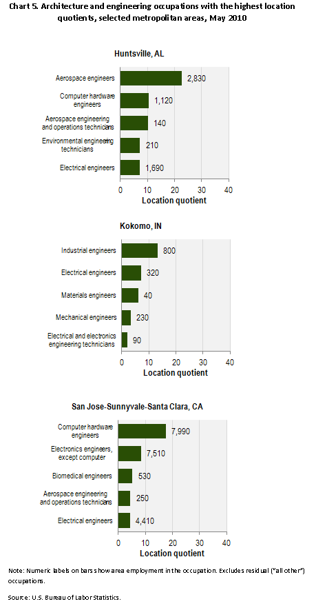
The employment share of architecture and engineering occupations varied even more by local area than by state. Metropolitan areas with the lowest shares of architecture and engineering occupations—less than 0.5 percent of employment—included Merced, CA; Vineland–Millville–Bridgeton, NJ; Visalia–Porterville, CA; and Punta Gorda, FL. At the other end of the spectrum, architecture and engineering occupations made up nearly 9 percent of employment in Huntsville, AL; nearly 7 percent of employment in Kokomo, IN; and about 6 percent of employment in San Jose–Sunnyvale–Santa Clara, CA; Kennewick–Pasco–Richland, WA; and Palm Bay–Melbourne–Titusville, FL.
Architecture and engineering occupations with the highest location quotients in the Huntsville, Kokomo, and San Jose areas are shown in chart 5. Aerospace engineers had both the highest location quotient (22.6) and highest employment (2,830) of any architecture and engineering occupation in Huntsville. Other architecture and engineering occupations with high location quotients in this area included computer hardware engineers and aerospace engineering and operations technicians. Like Michigan, Kokomo, IN, had high concentrations of several occupations associated with manufacturing, including industrial engineers, materials engineers, and mechanical engineers. San Jose had both the highest employment (7,990) and highest location quotient (17.7) of any area for computer hardware engineers. Other engineering occupations with above-average concentrations in San Jose were electronics engineers, except computer; biomedical engineers; aerospace engineering and operations technicians; and electrical engineers.
San Jose–Sunnyvale–Santa Clara was also one of the highest paying areas overall for architecture and engineering occupations, with an annual mean wage of $100,750, more than $25,000 above the U.S. average for this group. Chart 6 shows mean wages for architecture and engineering occupations, along with the difference from the U.S. average for this group, for other high- and low-paying metropolitan areas.
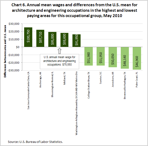
In general, the lowest paying areas for architecture and engineering occupations tended to be smaller metropolitan areas with below-average concentrations of these occupations. For example, the low-paying areas shown in chart 6 had overall employment ranging from 16,960 in Palm Coast, FL, to 123,680 in Brownsville–Harlingen, TX; of the areas shown, only College Station–Bryan, TX, had an above-average share of architecture and engineering jobs. The picture is more mixed for the highest paying areas. Some, such as San Jose or the Washington, DC, metropolitan division, were large metropolitan areas that were more likely to have above-average wages in general. Others, including Midland, TX, with overall employment of 64,210, were smaller areas. However, in general, areas with higher concentrations of architecture and engineering occupations also had higher wages for this group.
Within a given metropolitan area, average wages for the architecture and engineering group were affected by both the wages for individual occupations and the relative shares of high- and low-paying occupations within the group. San Jose, for example, had above-average wages for nearly all of the area’s architecture and engineering occupations for which wage estimates were available. In many cases, the differences were large; for instance, the mean wage for biomedical engineers in San Jose was $30,780 higher than the U.S. average for the occupation, and the mean wage for chemical engineers was $27,250 higher than average. In contrast, most architecture and engineering occupations in Midland, TX, had wages below or similar to their respective U.S. averages, but nearly 46 percent of Midland’s architecture and engineering employment consisted of petroleum engineers, typically one of the highest paying occupations in the group.
Data profiles of architecture and engineering occupations are available from the OES occupational profiles page. Complete Occupational Employment Statistics data for May 2010 are available from the OES home page. This highlight was prepared by Audrey Watson. For more information, please contact the OES program.
Last Modified Date: February 8, 2012