
An official website of the United States government
An official website of the United States government
The .gov means it's official.
Federal government websites often end in .gov or .mil. Before sharing sensitive information,
make sure you're on a federal government site.
The site is secure.
The
https:// ensures that you are connecting to the official website and that any
information you provide is encrypted and transmitted securely.

Crossref 0
Changes in Wages and Occupational Mix of Fourth District Metro Areas Between 2019 and 2022, Changes in Wages and Occupational Mix of Fourth District Metro Areas Between 2019 and 2022, 2024.
In this article, we describe the details of an alternative estimation method for producing estimates of occupational employment levels and mean wages for the Occupation Employment Statistics survey. In addition, we introduce a bootstrap variance estimation system to accompany the new estimation method. A comparison of the official May 2016 estimates with our model-based estimates shows general agreement between the two sets of estimates.
The Occupational Employment Statistics (OES) survey measures occupational employment levels and wage rates for wage and salary workers in nonfarm establishments in the 50 states, the District of Columbia, Guam, Puerto Rico, and the Virgin Islands. Estimates of occupational employment and wage rates are based on six panels of survey data collected over a 3-year cycle. The final in-scope sample size when six panels are combined is approximately 1.2 million establishments.
A well-known drawback of the 3-year sample design is the data users’ inability to efficiently compare estimates from year to year. Such an ability is critical to developing an understanding of the changing demand for occupations in the labor market. To improve data users’ ability to make year-to-year comparisons, the U.S. Bureau of Labor Statistics (BLS) initiated a long-term research project that resulted in a recommendation for a new sample design and estimation method. A comprehensive simulation study showed that the new sample design and estimation method substantially improved the accuracy and reliability of the estimates as well as the ability of data users to make efficient year-to-year comparisons. Although a new sample design has not been implemented, BLS decided to test whether the new estimation method could yield improvements over the current estimation method without changing the sample design. Testing indicated that the accuracy and reliability of the estimates improved greatly over the current approach, so BLS decided to publish several years of data using the new estimation method as a research series.1
This article describes the details of the new estimation method under the current sample design. We first begin by discussing the key features of the OES sample design that are particularly relevant for the new estimation method. We then present the new estimation method. Next, because the new estimation method requires a different method for estimating variances, we present the details of a new variance estimation methodology. Finally, we conclude the article with some comparisons of estimates produced using the current estimation method and the alternative estimation method.
The current OES estimation methods require that data from a minimum number of sample units be used for each estimate (or estimation cell). In order for the sample to meet this requirement, the current sample design stratifies the sampling frame into nearly 170,000 detailed-area by detailed-industry strata. A large sample is required to provide sample coverage for the 170,000 strata. For practical reasons, the number of sample units required for OES cannot be collected within a single period. For this reason, the OES sample is selected and collected on the basis of a 3-year survey cycle, in which approximately 200,000 establishments are sampled biannually in May and November. These biannual samples are called panel samples. The establishments selected in any given panel are excluded from selection in the next five panels. The exception to this rule is federal and state government establishments; a census of these units is collected yearly. To provide adequate geographical, industrial, and occupational coverage, OES combines 3 years of panel samples to produce estimates. The current sample designs complete this process by using a rolling six-panel cycle, in which a current panel sample is rolled in to replace an older panel sample selected 3 years prior. Approximately 1.2 million sampled establishments are used for any given set of estimates.
Each OES panel sample is selected with the use of a stratified design, in which strata are defined by state, detailed area, aggregate North American Industry Classification System (NAICS) industry, and ownership for schools, hospitals, and gambling establishments. 2 Each stratum is divided into two substrata based on whether an establishment’s employment is below or above a predetermined threshold. The substratum containing the larger establishments are selected with certainty into the OES panel sample. Only the establishments in the certainty stratum that were not sampled in the previous five panels are included in the current panel sample. The establishments in the substratum containing the smaller establishments are selected into the OES sample with the use of a probability sample. The number of sample units selected in each noncertainty stratum is determined by two different allocation schemes. The first scheme simply allocates a minimum number of sample units on the basis of the number of establishments found within the stratum. The second scheme uses the employment levels and a measure of the occupational variability to determine the number of sample units to allocate to the stratum. The occupational variability measure is calculated with the use of past OES microdata and is assigned to each aggregate NAICS industry. More sample is allocated to noncertainty strata that contain a larger number of employees and a larger measure of occupational variability. The final allocation for each noncertainty stratum is the maximum number of units allocated between the two allocations.
Within each noncertainty stratum, establishments are selected into the OES panel sample with probability proportionate to their employment. Larger establishments are given higher probabilities of selection than smaller establishments. OES uses special techniques to ensure that establishments that were selected in any of the five previous panels are not selected into the current panel. A sampling weight equal to the inverse of the selection probability is assigned to each selected establishment. The sampling weights can be used to weight up the OES panel sample to represent the target population that the sample was selected from.
OES combines six OES panel samples to calculate the OES estimates. Special adjustments are needed so that the combined six panel sample properly weights up to the population. For the certainty sample units, the final sampling weight is set to 1. For the noncertainty sample, the final sampling weight is equal to the panel sample weight divided by the number of times its stratum is represented in the six panels. For example, suppose a particular noncertainty stratum is found in all six panels, meaning some sample was selected from that stratum in each of the six panels. Since each panel sample represents the entire population, the unadjusted weighted data for the six-panel sample would overrepresent the population by a factor of six. To ensure the six-panel sample more accurately represents the population, the current estimation methods divide the sampling weights of all the sampled units found in the stratum by six.
The six-panel weighted data represent the average population across the periods when each panel sample was selected. For the final estimates, the six-panel weighted data are benchmarked to the population corresponding to the reference period of the estimates.
The current estimation method is a version of a standard design-based estimator, modified to accommodate the complexities of the sample design. In contrast, the proposed model-based estimation method using 3 years of OES data, which we will refer to as MB3, attempts to leverage the information provided by sample respondents differently. The approach takes advantage of the fact that we observe key determinants of occupational staffing patterns and wages for all units in a target population. In particular, the Quarterly Census of Employment and Wages (QCEW) provides data on the detailed industry, ownership status, geographic location, and size for every establishment whose workers are covered by state unemployment insurance laws.
With the auxiliary QCEW data in mind, we developed our estimation method to predict the outcomes of interest, namely occupational staffing patterns and the associated wages, for every unit in the target population. Only a small minority of establishments provide direct reports of these outcomes. For the overwhelming majority, however, we need to predict or estimate these outcomes on the basis of the information provided by responding units. Therefore, the best way to think about our estimation method is by asking, “What is the best way to predict the staffing pattern and associated wages at a nonresponding establishment?”
A reasonable and somewhat obvious answer is by using a previously observed staffing pattern and wages from the same establishment. Provided that the establishment is roughly the same size as when it responded, the old staffing pattern is probably a good predictor of the current staffing pattern. This answer is especially true if establishments have idiosyncratic staffing patterns or consistently pay above or below prevailing market wages.
However, for establishments that have not responded to the OES survey in the recent past, we find it reasonable to predict the staffing patterns and wages by finding one or more responding establishments with similar characteristics to the nonresponding establishment. For estimating staffing patterns, we conject that detailed industry and employment size are the most important establishment characteristics, all else equal. We prefer to find establishments from the current sample and from the same detailed area as the nonresponding establishment.
With this in mind, we begin by describing the types of units the sampling and survey process yields and how we exploit not only current information but also previously collected information.
For each unit e in the target population, we observe the current employment level Ee and a vector of current establishment characteristics Xe that includes location (Metropolitan Statistical Area [MSA] or Balance of State [BOS] area), industry (six-digit NAICS), and ownership status (private, local government, or state government). We denote the set of establishments in the target population as Ω .
In addition to OES-specific occupational employment and wage information, every establishment that responds to the OES survey reports an employment level Ere and a vector of establishment characteristics X re that includes location, industry, and ownership status. We denote the set of establishments that responded to the OES survey over the past six panels as R.
For each responding establishment in the full six-panel OES sample that also exists in the current target population, we determine whether the information reported to the OES is similar to the information contained in the population database, the QCEW. To be specific, we define the set of stable responders S as
S = {e ∈ ∩ Ω: Ere is close enough to Ee and X re = Xe} .
This set therefore includes continuing units that responded to the survey over the past six panels whose reported location, industry, and ownership status are identical to the information contained in the QCEW and whose reported employment is similar to the current population employment. We define “close enough” employment in both an absolute and relative sense. In particular, we require that reported employment is within 50 percent or within five employees of the employment reported to the QCEW. For example, we consider an establishment close enough if it reports 100 employees to the OES but has 120 employees, according to the QCEW. On the other hand, we consider an establishment not close enough if it reports 20 employees to the OES but has 10 employees according to the QCEW.
Table 1 shows the percentage of responding units by collection panel that were deemed stable and unstable and the reason why the units were unstable for the May 2016 estimates. Not surprisingly, the percentage of stable units is higher in more recent panels, ranging from slightly more than 86 percent in the May 2014 panel to nearly 93 percent in the May 2016 panel. Employment differences are the major cause for units to be characterized as unstable, although industry code differences also cause instability in units, especially for older responders. However, ownership and MSA differences are not very common.
| Panel | Percent stable | Unstable reasons | |||
|---|---|---|---|---|---|
| NAICS difference | MSA difference | Ownership difference | Employment difference | ||
| 201602 | 93.23 | 0.97 | 0.40 | 0.03 | 5.59 |
| 201504 | 92.54 | 1.16 | 0.42 | 0.11 | 6.00 |
| 201502 | 91.79 | 1.93 | 0.86 | 0.18 | 5.87 |
| 201404 | 89.79 | 2.61 | 1.01 | 0.43 | 7.07 |
| 201402 | 89.47 | 3.08 | 0.90 | 0.36 | 7.22 |
| 201304 | 88.47 | 3.03 | 1.17 | 0.26 | 8.09 |
| Notes: The percentages across the columns do not sum to 100 because units can be unstable for more than one reason. MSA = Metropolitan Statistical Area and NAICS = North American Industry Classification System. Sources: U.S. Bureau of Labor Statistics and authors’ calculations. | |||||
We have now partitioned the target population into two groups: stable responders and all other units, which we will generically call nonresponders. We should note that the set of nonresponders includes three distinct groups—unstable responders, sampled nonresponders, and nonsampled units. The MB3 approach does not distinguish between the three groups. For these units, the prediction methods estimate the outcomes of interest by using data from units that responded to the survey over the past six panels.3 In contrast, the current OES approach clearly distinguishes between these three groups. In the current approach, unstable responders are treated exactly as stable responders, the outcomes for sampled nonresponders are imputed, and the outcomes of nonsampled units are implicitly estimated with the use of the weighted average of outcomes from sample units in their sampling strata.4
As just discussed, our estimation method relies on predicting the staffing patterns and corresponding occupational wages for unobserved population units by exploiting the information provided by responding units. In this sense, our estimation method is no different from the current approach in which information from sample units is implicitly used to predict the outcomes of nonsample units. The major deviation between our approach and the current approach is how we choose to weight responding units.
To understand the estimation method, consider a single nonresponding population unit with certain observed characteristics such as detailed industry, detailed area, ownership status, state, and current employment. The objectives of the estimation method are to find the responding units that are most similar to the nonresponding unit along these dimensions and to predict the outcomes of interest at this unit on the basis of the information provided by these responding units.
For practical purposes related to a computational burden, we choose to find potential matches from the set of responding units using a hierarchical structure that systematically relaxes how similar respondents must be to the nonresponding unit in terms of both employment and observable characteristics.
Table 2 below shows the criteria used for each level of the hierarchy. The first two levels of the hierarchy yield perfect matches to the nonresponding unit in terms of industry, ownership, and area and yield very similar levels of employment (within 10 percent in the highest level and within 20 percent in level 2). The first characteristic that we relax in the hierarchy is detailed area, but even matches in levels 3 and 4 of the hierarchy must be in the same state as the nonresponding unit. We then subsequently relax industry to aggregate industry, which is generally a four-digit NAICS industry, and eliminate the employment proximity condition. Our expectation is that an overwhelming majority of the nonresponding units will have been predicted by level 5 of the hierarchy.5
| Hierarchy level | Characteristics that must match between the nonresponding unit and donor | Employment criteria (relative, in percent, or absolute) |
|---|---|---|
| 1 | State, NAICS, ownership, and MSA | 10 or 3 |
| 2 | State, NAICS, ownership, and MSA | 20 or 5 |
| 3 | State, NAICS, and ownership | 10 or 3 |
| 4 | State, NAICS , and ownership | 20 or 5 |
| 5 | State, E_NAICS, and ownership | None |
| 6 | State and E_NAICS | None |
| 7 | NAICS and ownership | 10 or 3 |
| 8 | NAICS and ownership | 20 or 5 |
| 9 | NAICS | None |
| 10 | E_NAICS | 20 or 5 |
| 11 | E_NAICS | None |
| Notes: E_NAICS = estimation of North American Industry Classification System, NAICS = North American Industry Classification System, and MSA = Metropolitan Statistical Area. Sources: U.S. Bureau of Labor Statistics and authors’ calculations. | ||
In order for a nonresponding unit to be predicted at a particular hierarchy level, at least five responding units or donors must be available. This means, for example, in order for a nonresponding unit to be predicted at the highest level of the hierarchy, at least five responding units must be within the same state, six-digit NAICS, ownership status, and MSA and also be within 10 percent of the nonresponding unit’s current employment level.
Since we pool data across detailed areas, industries, establishment sizes, and time (up to six panels), we weight the data so that donors that are closer in both space (area, industry, ownership status, and employment) and time to the nonresponding unit get relatively more weight in the estimator.
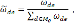
In particular, for nonresponding unit e the weight assigned to the responding unit or donor d is

where I is an indicator function that equals 1 if the argument is true and 0 otherwise. We denote reported donor characteristics with a d subscript and an r superscript, while an e subscript is used to denote nonresponding unit’s characteristics. The variable E represents employment level, k represents detailed industry, s represents ownership status, and z represents a vector of geographic characteristics, including detailed area, urban-rural status, and state. The variable pd represents the panel in which the donor responded to the OES survey. The variable can take values from 0 to 5, where 0 indicates the current panel, 1 indicates the previous panel, and so on. Finally, δ and δ are constants and δ is a function that relates the geographic proximity of the donor and the nonresponding unit to the weight.
The best way to think about the weighting function is as a set of penalties for deviating from a perfect match in our five observable dimensions. The weight achieves a maximum value of 1, if the reported employment level of the donor is the same as the employment level of the nonresponding unit; the detailed area, industry, and ownership status of the donor are the same as the nonresponding unit; and the donor responded to the OES in the current panel. Let us consider each penalty in turn. In addition, one should note that the particular value of the weight is not important, only the weight relative to the other donors matters.
The part of the weight attached to employment differences between the donor and the nonresponding unit attaches greater weight (or a smaller penalty) to larger donors when the absolute employment difference is the same. For example, consider a nonresponding unit with 11 workers. A donor with 1 worker will have a weight of  , while a donor with 21 workers will have a weight of
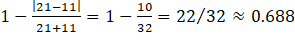 . The reason for the asymmetry in the employment difference penalty is that small establishments tend to employ few occupations and their staffing patterns do not accurately represent the staffing patterns of larger establishments. Note that as the employment of the nonresponding unit increases, the difference in the weights decreases between a smaller and larger donor, with employment levels equally different from the nonresponding unit. For example, consider a nonresponding unit with 100 workers. A donor reporting 90 workers will have an employment weight of
 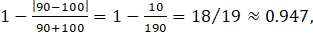 while a donor reporting 110 workers will have an employment weight of
 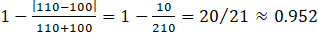 .
.
The weight associated with when the donor responded to the OES survey is monotonically decreasing in the age of the response. A current response gets a weight of 1 (i.e., no penalty), whereas a response from five panels earlier receives a weight of 1/6.
A donor that is not in the same detailed industry as the nonresponding unit gets a penalty of δ = 0.75 for every industry, except for detailed industries within the Employment Services industry in which the penalty increases to δ = 0.95. Note that since industry is critical in determining the staffing pattern of an establishment, donors are always in the same four-digit industry as the nonresponding unit. A donor that does not have the same ownership status as the nonresponding unit gets a penalty of δs = 0.5.
Finally, we penalize donors for their geographical dissimilarity to the nonresponding unit. If the donor and the nonresponding unit are located in the same detailed area, no penalty is imposed. If the donor and the nonresponding unit are in different detailed areas but are in the same state and share the same urban-rural status, a penalty of 1/4 is calculated. If the donor and the nonresponding unit have a different urban-rural status but are both located in the same state, a penalty of 1/2 is calculated. If the donor and the nonresponding unit are located in different states, a penalty of 3/4 is calculated.
To limit the size of datasets created during the estimation procedure and increase processing speed, we use only donors with the 10 largest weights for the prediction. We then compute relative MB3 weights using the top 10 donors as
where Me equals the set of the 10 best donors for nonresponding establishment e. It follows that ∑∈Me ῶde = 1.
Table 3 shows the amount of data predicted at each level of the hierarchy for the May 2016 estimates. The table also shows that nearly all (99.3 percent) employment in nonresponding establishments will be predicted from donors in the same state and four-digit industry. Moreover, we see that close to 60 percent of employment in nonresponding establishments will be predicted with the use of only similarly sized donors in the same state and detailed industry. An even greater share of nonresponding units is predicted at the first four levels of the hierarchy. Nearly 32 percent of nonresponding units are predicted with the use of only similarly sized donors from the same detailed area and detailed industry, while slightly more than 86 percent of nonresponding units are predicted with only similarly sized donors from the same state and detailed industry.
| Hierarchy level | Characteristics that must match between nonresponding unit and donor | Employment criteria (relative, in percent, or absolute) | Units predicted | Percent of total units predicted | Employment predicted | Percent of total employment predicted |
|---|---|---|---|---|---|---|
| 1 | State, NAICS, ownership, and MSA | 10 or 3 | 1,623,137 | 23.3 | 9,826,885 | 10.3 |
| 2 | State, NAICS, ownership, and MSA | 20 or 5 | 612,296 | 8.8 | 8,358,865 | 8.8 |
| 3 | State, NAICS, and ownership | 10 or 3 | 3,420,188 | 49.1 | 30,216,449 | 31.8 |
| 4 | State, NAICS, and ownership | 20 or 5 | 367,966 | 5.3 | 8,945,059 | 9.4 |
| 5 | State, E_NAICS, and ownership | None | 920,293 | 13.2 | 36,786,760 | 38.7 |
| 6 | State and E_NAICS | None | 1,717 | 0.0 | 226,100 | 0.2 |
| 7 | NAICS and ownership | 10 or 3 | 18,673 | 0.3 | 307,888 | 0.3 |
| 8 | NAICS and ownership | 20 or 5 | 1,015 | 0.0 | 112,085 | 0.1 |
| 9 | NAICS | None | 1,305 | 0.0 | 210,507 | 0.2 |
| 10 | E_NAICS | 20 or 5 | 25 | 0.0 | 683 | 0.0 |
| 11 | E_NAICS | None | 1 | 0.0 | 80 | 0.0 |
| Total | — | — | 6,966,616 | 100.0 | 94,991,361 | 100.0 |
| Notes: MSA = Metropolitan Statistical Area, E_NAICS = estimation of North American Industry Classification System, and NAICS = North American Industry Classification System. Dashes indicate no data. Sources: U.S. Bureau of Labor Statistics and authors’ calculations. | ||||||
Table 4 compares the current method to the MB3 method in terms of how much employment is estimated from respondents in each of the six panels. As expected, in the current method roughly one-sixth of the employment total comes from each of the six panels. However, in the MB3 method, the amount of estimated employment is decreasing in the age of the response. Data collected from the most current two panels account for 52 percent of total employment, whereas data collected from the final two panels only account for 15 percent of total employment. Since the MB3 weighting function favors donors from more recent panels, the MB3 estimates are based on more current data than the data of the current OES approach.
| Panel | OES | MB3 | ||
|---|---|---|---|---|
| Level | Percent of total | Level | Percent of total | |
| 2016Q2 | 22,923,335 | 17 | 39,320,054 | 29 |
| 2015Q4 | 23,541,521 | 17 | 31,823,187 | 23 |
| 2015Q2 | 23,330,799 | 17 | 25,717,972 | 19 |
| 2014Q4 | 21,620,260 | 16 | 17,673,073 | 13 |
| 2014Q2 | 22,611,595 | 16 | 13,149,587 | 10 |
| 2013Q4 | 23,028,642 | 17 | 9,041,105 | 7 |
| Total | 137,056,152 | 100 | 136,724,978 | 100 |
| Notes: State and federal government employment is excluded from these counts, since we received a census of these employees in the 2016Q2 and 2015Q4 panels. MB3 = model-based estimation using 3 years of OES data, OES = Occupational Employment Statistics, Q2 = second quarter, and Q4 = fourth quarter. Sources: U.S. Bureau of Labor Statistics and authors’ calculations. | ||||
The process just detailed identifies a set of OES responders or donors whose observed outcomes will be combined with the use of the relative MB3 weights to form the predicted outcomes for any nonresponding unit. Because the process involves combining information from donors that may vary in terms of reported employment size, detailed area, detailed industry, ownership status, and the age of the response (i.e., in what panel the donor responded), the observed outcomes of the various donors must be adjusted. This adjustment accounts for systematic wage differences over time and across areas and industries.
For example, the wages of a donor that matches the nonresponding unit perfectly but responded to the survey five panels prior to the current period will typically need to be positively adjusted so that wage inflation is accounted for. On the other hand, the wages of a donor that responded to the survey in the current period but is located in a detailed area that typically pays higher wages than the area where the nonresponding unit is located will typically need to be adjusted down so that the systematic differences in wage levels between the two areas are accounted for.
Before detailing our procedure for updating and localizing the wages of donors, we need to mention that the current OES estimation method also requires that wages collected in the five past panels be updated to the current panel’s reference period. The current method uses the Employment Cost Index (ECI) to adjust wages from prior panels before combining them with the current panel’s data. The ECI estimates are available for nine aggregate occupation groups in which each group consists of similar major Standard Occupational Classification (SOC) groups. The wage updating procedure adjusts each detailed occupation’s wage rate, as measured in the earlier panel, according to the average movement of its ECI occupation group nationally.
In contrast to the current approach, our method does not rely on data from other surveys. Instead, we choose to employ a regression technique that allows us to estimate occupation, area, industry by ownership, and employment size wage effects, as well as a major occupation group by panel wage effects. We are primarily interested in the estimated area wage effects and major occupation group by panel wage effects.6
Even after controlling for differences in occupational and industrial composition of areas, we find relatively large systemic differences in wage levels across geographic areas. Table 5 shows the 10 MSAs with the highest area wage effects and the 10 MSAs with the lowest area wage effects. Other things equal, the results suggest that wages in San Francisco are roughly 43 percent higher than wages in the baseline area of Charleston–North Charleston, South Carolina.7 Conversely, wages in Pine Bluff, Arkansas, are roughly 12 percent lower than wages in Charleston. Although incredibly unlikely, if an OES respondent that is located in San Francisco is used as a donor for a nonresponding unit located in Pine Bluff, Arkansas, the wages of the San Francisco unit would be adjusted downward by a factor of 0.8827/1.4345 » 0.6153.8
| MSA | MSA name | Estimated area wage effect |
|---|---|---|
| Top 10 | ||
| 41884 | San Francisco–Redwood City–South San Francisco, CA, metropolitan division | 1.4345 |
| 41940 | San Jose–Sunnyvale–Santa Clara, CA | 1.3964 |
| 42034 | San Rafael, CA, metropolitan division | 1.3787 |
| 36084 | Oakland–Hayward–Berkeley, CA, metropolitan division | 1.3139 |
| 35614 | New York–Jersey City–White Plains, NY–NJ, metropolitan division | 1.3069 |
| 34900 | Napa, CA | 1.3026 |
| 71950 | Bridgeport–Stamford–Norwalk, CT | 1.2952 |
| 71654 | Boston–Cambridge–Newton, MA, NECTA division | 1.2921 |
| 21820 | Fairbanks, AK | 1.2865 |
| 11260 | Anchorage, AK | 1.2861 |
| Bottom 10 | ||
| 38220 | Pine Bluff, AR | 0.8827 |
| 30020 | Lawton, OK | 0.8929 |
| 25620 | Hattiesburg, MS | 0.8932 |
| 22900 | Fort Smith, AR–OK | 0.8933 |
| 26300 | Hot Springs, AR | 0.8935 |
| 10780 | Alexandria, LA | 0.9033 |
| 15180 | Brownsville–Harlingen, TX | 0.9048 |
| 27860 | Jonesboro, AR | 0.9052 |
| 16060 | Carbondale–Marion, IL | 0.9083 |
| 13220 | Beckley, WV | 0.9099 |
| Notes: Charleston–North Charleston, SC (Metropolitan Statistical Area [MSA] = 167000), is the now the baseline MSA. NECTA = New England City and Town Area. Sources: U.S. Bureau of Labor Statistics and authors’ calculations. | ||
In addition, wage levels tend to systematically increase over time, even after occupation, industry, and area effects are controlled for. Similar to the current OES approach, our regression model allows the wages of occupation groups to evolve differently over time. Our regression model allows differences in wage growth rates for 22 major occupation groups, whereas the current approach uses nine ECI occupation groups. Table 6 shows the wage adjustments for the 22 major occupation groups from November 2013 to May 2016. By construction, no wage adjustments exist for the May 2016 data, so the adjustments all equal 1. Going back 1 year to data collected in May 2015, we see that, by and large, wages within major occupation groups grew between 1 percent and 4 percent. The wages of business and financial operations occupations, community and social service occupations, and protective service occupations grew by less than 1 percent, and the wages of life, physical, and social science occupations and farming, fishing, and forestry occupations grew by more than 4 percent. Going back 2 years to data collected in May 2014, we see that the wages of every major occupation group except farming, fishing, and forestry occupations grew between 2 percent and 8 percent.
| Major SOC code | SOC title | May 2016 | November 2015 | May 2015 | November 2014 | May 2014 | November 2013 |
|---|---|---|---|---|---|---|---|
| 11 | Management occupations | 1.000 | 1.032 | 1.040 | 1.040 | 1.064 | 1.060 |
| 13 | Business and financial operations occupations | 1.000 | 1.029 | 0.997 | 1.005 | 1.031 | 1.026 |
| 15 | Computer and mathematical occupations | 1.000 | 1.026 | 1.012 | 1.034 | 1.034 | 1.039 |
| 17 | Architecture and engineering occupations | 1.000 | 1.002 | 1.021 | 1.003 | 1.035 | 1.038 |
| 19 | Life, physical, and social science occupations | 1.000 | 1.088 | 1.051 | 1.077 | 1.071 | 1.121 |
| 21 | Community and social services occupations | 1.000 | 0.992 | 1.005 | 1.020 | 1.044 | 1.047 |
| 23 | Legal occupations | 1.000 | 1.018 | 1.040 | 1.021 | 1.024 | 1.008 |
| 25 | Education, training, and library occupations | 1.000 | 1.020 | 1.031 | 1.042 | 1.059 | 1.062 |
| 27 | Arts, design, entertainment, sports, and media occupations | 1.000 | 0.979 | 1.003 | 1.026 | 1.039 | 1.053 |
| 29 | Healthcare practitioners and technical occupations | 1.000 | 1.014 | 1.014 | 1.013 | 1.037 | 1.038 |
| 31 | Healthcare support occupations | 1.000 | 1.005 | 1.021 | 1.023 | 1.047 | 1.044 |
| 33 | Protective service occupations | 1.000 | 0.960 | 0.979 | 1.011 | 1.034 | 1.059 |
| 35 | Food preparation and serving related occupations | 1.000 | 1.018 | 1.023 | 1.042 | 1.068 | 1.086 |
| 37 | Building and grounds cleaning and maintenance occupations | 1.000 | 1.018 | 1.031 | 1.040 | 1.071 | 1.068 |
| 39 | Personal care and service occupations | 1.000 | 1.007 | 1.018 | 1.044 | 1.054 | 1.064 |
| 41 | Sales and related occupations | 1.000 | 1.019 | 1.032 | 1.034 | 1.054 | 1.060 |
| 43 | Office and administrative support occupations | 1.000 | 1.016 | 1.023 | 1.039 | 1.051 | 1.055 |
| 45 | Farming, fishing, and forestry occupations | 1.000 | 1.016 | 1.076 | 1.057 | 1.108 | 1.112 |
| 47 | Construction and extraction occupations | 1.000 | 1.011 | 1.026 | 1.034 | 1.043 | 1.063 |
| 49 | Installation, maintenance, and repair occupations | 1.000 | 0.998 | 1.021 | 1.015 | 1.040 | 1.033 |
| 51 | Production occupations | 1.000 | 1.007 | 1.033 | 1.052 | 1.057 | 1.066 |
| 53 | Transportation and material moving occupations | 1.000 | 1.025 | 1.039 | 1.057 | 1.067 | 1.072 |
| Note: SOC = Standard Occupational Classification. Sources: U.S. Bureau of Labor Statistics and authors’ calculations. | |||||||
In addition to the model allowing for primary adjustments made for geographic wage differences and wage differences over time, the model allows for adjustments because of industry, ownership, and employer size differences. These effects tend to be small relative to the geographic and sample period effects.
With the wage adjustments and relative MB3 weights in hand, we can simply update and combine OES-specific information provided by donors to predict the outcomes of interest at the nonresponding establishment. We explain this process by tracing through the entire MB3 estimation process for a single nonresponding unit in the May 2016 population. In particular, the unit employs 100 workers and is located in the Allentown–Bethlehem–Easton, PA, MSA.9
Table 7 shows the establishment characteristics and associated weights for the five donors available for this nonresponding unit. For example, the first donor reported data in the May 2016 survey; is located in the Lancaster, PA, MSA; is in the same six-digit industry as the nonresponding unit; and employs 101 workers. Since the first donor is in the current panel and in the same detailed industry as the nonresponding unit, the panel and industry weights both equal 1. Because the donor is in a different MSA, but in the same state and urban-rural status as the nonresponding unit, the area weight is 3/4. Finally, since the employment level of the donor is nearly identical to the nonresponding unit, the employment weight is nearly 1 at 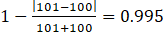 . Multiplying the four weights yields an MB3 weight of 0.746. Similarly, we construct MB3 weights for the other four donors.
| Variable | Donor | ||||
|---|---|---|---|---|---|
| 1 | 2 | 3 | 4 | 5 | |
| Sample panel | May 2016 | May 2016 | November 2015 | May 2015 | November 2014 |
| Panel weight | 1 | 1 | 5/6 | 4/6 | 3/6 |
| MSA | Lancaster, PA | Allentown–Bethlehem–Easton, PA | Lebanon, PA | Montgomery County–Bucks County–Chester County, PA | Reading, PA |
| Area weight | 3/4 | 1 | 3/4 | 3/4 | 3/4 |
| Level of industry match | 6 digit | 6 digit | 6 digit | 6 digit | 6 digit |
| Industry weight | 1 | 1 | 1 | 1 | 1 |
| Employment | 101 | 45 | 87 | 89 | 65 |
| Employment weight | 0.995 | 0.621 | 0.93 | 0.942 | 0.788 |
| MB3 weight | 0.746 | 0.621 | 0.582 | 0.471 | 0.295 |
| Relative MB3 weight | 0.275 | 0.229 | 0.214 | 0.173 | 0.109 |
| Notes: MB3 = model-based estimation using 3 years of Occupational Employment Statistics data and MSA = Metropolitan Statistical Area. Sources: U.S. Bureau of Labor Statistics and authors’ calculations. | |||||
Recall that the goal of the MB3 estimation process is to predict the OES-specific outcomes of nonresponding units. The predictions are weighted sums (or averages) of the observed outcomes of the donors. Therefore, we divide the MB3 weights by the sum of the MB3 weights (over the five donors) so that the relative MB3 weights sum to 1. The nonresponding unit is represented by the weighted sum of the five donors. In our particular example, the first donor accounts for 27.5 percent of the unit, the second donor accounts for 22.9 percent of the unit, and so on. Therefore, the predicted outcomes for the nonresponding unit will be based largely on the outcomes of the first two donors because they represent slightly more than 50.0 percent of the nonresponding unit.
Table 8 presents the OES-specific information reported by the five donors. We present employment level, share of total establishment employment, and mean wages for three detailed occupations and the employment level for all other occupations. For example, donor 1 reported 19 workers in occupation 1. These 19 workers represent approximately 19 percent of the 101 total workers employed at this establishment. The mean wage paid to workers in occupation 1 by donor 1 is $20.28.
| Variable | Donor | ||||||
|---|---|---|---|---|---|---|---|
| 1 | 2 | 3 | 4 | 5 | |||
| Establishment employment | 101 | 45 | 87 | 89 | 65 | ||
| Sample panel | May 2016 | May 2016 | November 2015 | May 2015 | November 2014 | ||
| Relative MB3 weight | 0.275 | 0.229 | 0.214 | 0.173 | 0.109 | ||
| Area wage adjustment | 1.02 | 1.00 | 1.04 | 0.94 | 0.99 | ||
| Occupation 1 | |||||||
| Employment level | 19 | 14 | 0 | 30 | 25 | ||
| Employment share | 0.19 | 0.31 | 0.00 | 0.34 | 0.38 | ||
| Mean wage | $20.28 | $20.15 | — | $19.01 | $17.23 | ||
| Occupation division by panel adjustment | 1.00 | 1.00 | — | 1.03 | 1.06 | ||
| Adjusted employment level | 18.81 | 31.11 | 0.00 | 33.71 | 38.46 | ||
| Adjusted mean wage | $20.65 | $20.15 | — | $18.41 | $18.17 | ||
| Predicted employment level | 22.32 | ||||||
| Predicted mean wage | $19.44 | ||||||
| Occupation 2 | |||||||
| Employment level | 8 | 6 | 8 | 21 | 0 | ||
| Employment share | 0.08 | 0.13 | 0.09 | 0.24 | 0.00 | ||
| Mean wage | $17.10 | $18.45 | $15.17 | $16.98 | — | ||
| Occupation division by panel adjustment | 1.00 | 1.00 | 1.01 | 1.03 | — | ||
| Adjusted employment level | 7.92 | 13.33 | 9.20 | 23.60 | 0.00 | ||
| Adjusted mean wage | $17.41 | $18.45 | $15.87 | $16.45 | — | ||
| Predicted employment level | 11.29 | ||||||
| Predicted mean wage | $17.07 | ||||||
| Occupation 3 | |||||||
| Employment level | 11 | 0 | 0 | 3 | 8 | ||
| Employment share | 0.11 | 0.00 | 0.00 | 0.03 | 0.12 | ||
| Mean wage | $21.35 | — | — | $19.03 | $21.45 | ||
| Occupation division by panel adjustment | 1.00 | — | — | 1.02 | 1.04 | ||
| Adjusted employment level | 10.89 | 0.00 | 0.00 | 3.37 | 12.31 | ||
| Adjusted mean wage | $21.74 | — | — | $18.25 | $22.19 | ||
| Predicted employment level | 4.92 | ||||||
| Predicted mean wage | $21.45 | ||||||
| All other occupations | |||||||
| Employment level | 63 | 25 | 79 | 35 | 32 | ||
| Employment share | 0.62 | 0.56 | 0.91 | 0.39 | 0.49 | ||
| Adjusted employment level | 62.38 | 55.56 | 90.8 | 39.33 | 49.23 | ||
| Predicted employment level | 61.48 | ||||||
| Notes: MB3 = model-based estimation using 3 years of OES data and OES = Occupational Employment Statistics. Dashes indicate no data. Sources: U.S. Bureau of Labor Statistics and authors’ calculations. | |||||||
Since the nonresponding unit employs 100 workers, we simply multiply the employment share by 100 to predict the adjusted employment level in each of the occupations for each of the donors. For example, since the employment share of occupation 1 at donor 2 is 0.31, donor 2 predicts 31.11 workers in occupation 1. On the other hand, since donor 3 employs 0 workers in occupation 1, donor 3 predicts 0 workers in occupation 1. The weighted (by relative MB3 weights) sum of adjusted employment levels yields the final predicted employment level for the nonresponding unit. In our example, we predict 22.32 workers in occupation 1, 11.29 workers in occupation 2, 4.92 workers in occupation 3, and 61.48 workers in all other occupations. Obviously, these predictions sum to 100 so that employment of the nonresponding unit is completely accounted for.
Turning to predicted wages, we recognize that 4 of the 5 donors are located in different areas than the nonresponding unit and 3 of the 5 donors responded to the OES in panels prior to May 2016. Therefore, we must adjust reported wages to represent the wages that would be paid by an employer in the Allentown–Bethlehem–Easton, PA, MSA in May 2016.10
The area wage adjustment is constant across all occupations employed by a donor. For example, other things equal, the wages paid in Lancaster, PA (the location of donor 1), are typically slightly lower than the wages paid in Allentown–Bethlehem–Easton, PA (the location of the nonresponding unit). Therefore, the reported wages of donor 1 are multiplied by an area adjustment factor of 1.02. However, since the wages paid in Montgomery County–Bucks County–Chester County, PA (the location of donor 4), are typically higher than the wages paid in Allentown–Bethlehem–Easton, PA, the reported wages of donor 4 are multiplied by an area adjustment factor of 0.94.
As we just discussed, the wage inflation rate is allowed to vary by major occupation group. In our example, occupation 1 and occupation 2 are in the same major occupation group, whereas occupation 3 is in a different major occupation group. Obviously, the wages of the first two donors are not adjusted since they are reported in the current period. Since donor 4 responded in the May 2015 panel, reported wages are adjusted upward. For occupations 1 and 2, the wages are multiplied by 1.03, whereas the wages in occupation 3 are multiplied by 1.02. Since donor 5 responded in the November 2014 panel, we multiply the reported wages by slightly higher major occupation group and panel wage adjustments to account for any additional wage growth from November 2014 to May 2015.
For each detailed occupation, we multiply the reported mean wages by the area wage adjustment and the major occupation group by panel adjustment, and the results are shown in the rows labeled “Adjusted mean wage” in table 8. We estimate the final predicted mean wage for the nonresponding unit by first computing the total wages paid to an occupation by a donor (i.e., the product of adjusted mean wage and adjusted employment level), computing the total wages paid by the nonresponding unit using the weighted (by relative MB3 weights) sum of total wages in an occupation at a donor, and finally by dividing by the predicted employment level. Obviously the predicted mean wage is going to fall between the highest and lowest adjusted mean wages of the five donors.
We use a bootstrap variance estimator for estimating the variability of the MB3 occupational employment and wage estimates. The major appeal of the bootstrap variance estimator is that the MB3 estimation methods can be used directly for calculating each set of replicate estimates. Other replication techniques, such as the jackknife or balance repeated replication, require the sampling weights be adjusted for calculating the replicate estimates. This adjustment would be difficult under the MB3 methods since no single weight is associated with a respondent for estimation, but rather many weights are assigned to each respondent, depending on how the respondent is used. For example, a respondent can be used to predict itself and also be used as a donor in many different predictions. In these different situations, the respondent is assigned a different weight. This type of estimation does not lend itself well to the other common replication methods.
Each set of replicate estimates are based on a subsample of the full sample. We draw the subsample from the full sample using a stratified simple random sample with replacement design, in which the size of the subsample is equal to the size of the full sample. By sampling with replacement, we are essentially up-weighting some respondents by including them more than once in the subsample while down-weighting others by not including them at all. Subsampling only occurs for the noncertainty sample units. All certainty units from the full sample are used in every replicate’s bootstrap sample. We select six independent subsamples, one from each of the six biannual OES panel samples. The stratification plan is the same used for drawing the full sample, where strata are defined by state, MSAs, aggregate NAICS industry,11 and ownership for schools and hospitals.
In some situations, only one noncertainty sample unit is in each panel sample for a stratum. This results in selecting the same noncertainty sample units into the bootstrap subsample for each replicate, causing no variability to be measured for the stratum, which would result in a negative bias being introduced into the variance estimates. To remedy potential problems, we use a collapsing algorithm that ensures there are two or more noncertainty sample units to subsample from for the bootstrap sample.
The six bootstrap samples are combined for calculating the replicate MB3 estimates. The sampling weights assigned during the full sample are used in the replicate estimation. It is important to note that sampling weights are only used within the MB3 methods for calculating the wage interval means and the wage adjustment factors. The MB3 methods use the six-panel bootstrap sample for predicting occupational outcomes for all employees in the population, which is then used for calculating the MB3 replicate estimates. This process is repeated 300 times to create 300 sets of replicate estimates. We calculate the variance estimates by finding the variability across the occupational replicate estimates so that
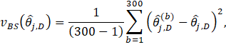
where  occupational estimate (employment or mean wage) for occupation j within estimation domain D, based on the full sample;
  occupational replicate estimates (employment or mean wage) for occupation , within estimation domain D based on the bootstrap subsample for replicate b.
We note that we are calculating the variance using the difference between the replicate estimate and the estimate from the full sample. This choice yields a more conservative estimate of the variance than an alternative approach, which instead uses the difference between the replicate estimate and the average of the replicate estimates in the variance formula.
The first set of research MB3 estimates has a reference period of May 2016. These estimates are directly comparable with the official May 2016 OES estimates. By comparing the MB3 research estimates with the official estimates, we are able to accomplish a few different goals. First, we are able to use the official OES estimates to check the new MB3 methods. We expect the current OES methods and MB3 methods to produce similar estimates at the lowest level of detail, since they are both estimating the same target population at the same reference period. As the level of comparison becomes more detailed, we expect the relative differences between the official and MB3 estimates to increase. Second, by finding where the official and MB3 estimates differ, we can understand how key differences in the current and MB3 methods are affecting the estimates. Third, by comparing the official and MB3 percent relative standard errors (PRSEs), we are able to determine which method produces more stable estimates.
The official and MB3 research estimates are calculated at many domains, varying in the level of geographic, industry, ownership, and occupation detail. In this section, we will limit our comparison with the following five estimation domains:
In the first subsection, we compare the occupational employment estimates; in the second, the occupational mean hourly wage estimates; and in the third, the PRSEs. We limit our comparison to estimates that would be published under both the current and MB3 methods according to the current confidentiality and quality screening rules.
In figure 1, we compare the official and MB3 national major group SOC occupational employment estimates using a scatter plot in which the official estimate is on the horizontal axis and the MB3 estimate is on the vertical axis. This level is the highest of occupational estimates that OES produces. Every estimate falls very close to the red 45-degree line, which indicates that the official and MB3 national major group employment estimates are quite similar. With the scale of this plot, we find that determining the magnitude of any differences is difficult, especially for the smallest employment estimates. Therefore, we show a more detailed comparison of the employment estimates in table 9.

| Estimation domain | Number of estimates | Comparison measure | 5th percentile | 10th percentile | 25th percentile | Median | 75th percentile | 90th percentile | 95th percentile |
|---|---|---|---|---|---|---|---|---|---|
| National major group SOC occupation | 22 | Employee difference | –120,979 | –93,828 | –36,202 | –11,433 | 23,262 | 61,112 | 76,294 |
| Employee percent difference | –2.7 | –2.1 | –0.8 | –0.2 | 0.6 | 1.1 | 1.2 | ||
| National by detailed SOC occupation | 818 | Employee difference | –10,612 | –5,199 | –2,145 | –172 | 1,158 | 5,077 | 9,293 |
| Employee percent difference | 15.4 | –10.9 | –4.8 | –0.6 | 2.5 | 6.6 | 11.2 | ||
| State by detailed SOC occupation | 33,867 | Employee difference | –656 | –336 | –91 | –2 | 75 | 307 | 632 |
| Employee percent difference | –34.3 | –24.5 | –10.7 | –0.3 | 9.6 | 26.4 | 42.7 | ||
| MSA by detailed SOC occupation | 173,358 | Employee difference | –216 | –109 | –31 | 0 | 29 | 94 | 181 |
| Employee percent difference | –36.6 | –27.1 | –12.7 | 0.3 | 16 | 40.9 | 66.3 | ||
| NAICS4 by detailed SOC occupation | 34,624 | Employee difference | –558 | –263 | –69 | –4 | 52 | 232 | 500 |
| Employee percent difference | –42.1 | –31.6 | –15.8 | –1.4 | 13.3 | 38.3 | 61.6 | ||
| Notes: MB3 = model-based estimation using 3 years of OES data, MSA = Metropolitan Statistical Area, NAICS4 = four-digit North American Industry Classification System, and SOC = Standard Occupational Classification. Sources: U.S. Bureau of Labor Statistics and authors’ calculations. | |||||||||
In figures 2–5, we compare estimates at the four additional domains. In each of the figures’ scatter plots, most of the points are concentrated close to the 45-degree line, showing that the current and MB3 methods tend to produce similar estimates across the different domains. But, as the detail level of the estimates increases, more noise appears in the scatter plots. These plots also show that no systematic differences appear between the official and MB3 estimates, since the points of the scatter plots fall symmetrically above and below the 45-degree line. Similar to figure 1, the scale of these plots makes determining the amount of the employment difference impossible.


In table 9, we provide descriptive statistics of the distribution of the employment estimate differences and percent differences across the five different estimation domains. The percent difference statistics confirm that the differences, relative to the size of the estimate, are increasing as the estimation domains becomes more detailed. For the least detailed domain, national by major group occupation, 90 percent of the estimates have a percent difference that falls between −2.7 percent (the 5th percentile) and 1.2 percent (the 95th percentile). For the most detailed domain, detailed occupation by MSA, 90 percent of the estimates have a percent difference that falls between −36.6 percent and 66.3 percent.
Figures 6–10 present plots that compare mean hourly wage estimates. These plots are similar to the employment estimate comparisons plots. The official and MB3 national major group occupation wage estimates are very similar; all the estimate pairs fall very close to the 45-degree line. The wage plot estimates are similar to the employment estimates in that as the level of detail increases, the more the estimates tend to differ. Another interesting result that the plots reveal is a systematic difference between the highest mean wage estimates. The MB3 mean hourly wage estimates are almost always higher than the official mean hourly wage estimates for detailed occupations with the highest hourly wages (about $100 and above).
 for national major SOC occupation, May 2016")
 for national detailed SOC occupation, May 2016")
 for state, by detailed SOC occupation, May 2016")
 for Metropolitan Statistical Area, by detailed SOC occupation, May 2016")
 for NAICS4, by detailed SOC occupation, May 2016")
To understand why MB3 estimates are systematically higher than official estimates for high wage occupations, we must first describe how the OES wages are collected. The OES program collects wage data in 12 nonoverlapping wage intervals. The respondent reports how many employees within an occupation are found in each wage interval. When OES hourly wage rates are estimated, a wage interval mean is assigned to all employees within each wage interval. The current and MB3 methods use different assumptions when calculating the wage interval means, especially for the highest wage interval. Every employee within the highest wage interval is assigned the same wage interval mean under the current methods, essentially setting an upper limit on the mean hourly wage estimates. In the MB3 methods, the wage interval mean for the upper interval can vary, depending on the area and occupation of the employees found in the interval. For this reason, the upper limit on the mean hourly wage estimate in MB3 is higher and is reached less often than the limit in the current methods.12
In table 10, we provide descriptive statistics of the distribution of the differences and percent differences for the mean wage estimates across the five estimation domains. Similar to the patterns of the employment estimates, the differences between the official and MB3 wage estimates increase as the domain detail increases. However, most of the percent differences found in table 10 are much smaller than those in table 9, meaning that the wage estimates tend to be more similar than the employment estimates between the two methods. For the least detailed domain, national by major group occupation, 90 percent of the wage estimates have a percent difference that falls between −2.9 percent and 2.0 percent. For the most detailed domain, detailed occupation by MSA, 90 percent of the estimates have a percent difference that falls between −14.9 percent and 16.0 percent.
| Estimation domain | Number of estimates | Comparison measure | 5th percentile | 10th percentile | 25th percentile | Median | 75th percentile | 90th percentile | 95th percentile |
|---|---|---|---|---|---|---|---|---|---|
| National major group SOC occupation | 22 | Wage difference | –$0.85 | –$0.81 | –$0.37 | –$0.14 | $0.00 | $0.12 | $0.70 |
| Wage percent difference | –2.9 | –2.2 | –1.8 | –0.7 | 0.0 | 0.7 | 2.0 | ||
| National detailed SOC Occupation | 821 | Wage difference | –$1.54 | –$0.98 | –$0.44 | –$0.11 | $0.20 | $0.80 | $1.48 |
| Wage percent difference | –5.0 | –3.7 | –1.9 | –0.5 | 0.9 | 3.0 | 5.0 | ||
| State by detailed SOC occupation | 35,458 | Wage difference | –$3.26 | –$2.07 | –$0.83 | –$0.11 | $0.51 | $1.72 | $3.01 |
| Wage percent difference | –11.6 | –8.0 | –3.7 | –0.6 | 2.3 | 6.9 | 11.2 | ||
| MSA by detailed SOC occupation | 188,175 | Wage difference | –$4.29 | –$2.65 | –$1.00 | –$0.07 | $0.81 | $2.38 | $3.99 |
| Wage percent difference | –14.9 | –10.4 | –4.7 | –0.4 | 4.1 | 10.5 | 16.0 | ||
| NAICS4 by detailed SOC occupation | 38,276 | Wage difference | –$4.83 | –$3.15 | –$1.32 | –$0.16 | $0.85 | $2.71 | $4.51 |
| Wage percent difference | –16.3 | –11.5 | –5.4 | –0.8 | 3.6 | 10.2 | 15.8 | ||
| Notes: MB3 = model-based estimation using 3 years of OES data, MSA = Metropolitan Statistical Area, NAICS4 = four-digit North American Industry Classification System, and SOC = Standard Occupational Classification. Sources: U.S. Bureau of Labor Statistics and authors’ calculations. | |||||||||
The last comparison we make is between the official and MB3 PRSEs. In table 11, we present descriptive statistics of the distribution of the ratio of the MB3 PRSE to the official PRSE for each of the five estimation domains. A ratio less than 1 indicates the MB3 estimate has a lower PRSE than the official estimate. The table contains the results for both the employment and mean wage PRSEs comparison ratios. In almost all situations, the MB3 approach has more estimates with a lower PRSE than the official estimates. The only exception is for the national major group wage estimates where at least 75 percent of the estimates have a lower PRSE under the current method than in the MB3 methods. Interestingly, at least 90 percent of the national major group employment estimates have a lower PRSE under the MB3 method than in the current methods. These results have no clear explanation, but we should mention that the PRSEs under both methods are very low, the majority being less than 0.5 percent.
| Estimation domain | Comparison measure | 5th percentile | 10th percentile | 25th percentile | Median | 75th percentile | 90th percentile | 95th percentile |
|---|---|---|---|---|---|---|---|---|
| National major group SOC occupation | Employment PRSE ratio | 0.44 | 0.55 | 0.62 | 0.74 | 0.90 | 1.02 | 1.21 |
| Wage PRSE ratio | 0.65 | 0.79 | 1.06 | 1.30 | 1.47 | 1.97 | 2.17 | |
| National detailed SOC occupation | Employment PRSE ratio | 0.38 | 0.52 | 0.70 | 0.90 | 1.12 | 1.33 | 1.56 |
| Wage PRSE ratio | 0.34 | 0.48 | 0.72 | 0.95 | 1.17 | 1.47 | 1.67 | |
| State by detailed SOC occupation | Employment PRSE ratio | 0.26 | 0.41 | 0.63 | 0.89 | 1.19 | 1.61 | 2.04 |
| Wage PRSE ratio | 0.17 | 0.31 | 0.58 | 0.88 | 1.21 | 1.65 | 2.03 | |
| MSA by detailed SOC occupation | Employment PRSE ratio | 0.19 | 0.25 | 0.37 | 0.56 | 0.84 | 1.27 | 1.72 |
| Wage PRSE ratio | 0.19 | 0.26 | 0.40 | 0.60 | 0.89 | 1.30 | 1.67 | |
| NAICS4 by detailed SOC occupation | Employment PRSE ratio | 0.24 | 0.40 | 0.67 | 0.94 | 1.25 | 1.62 | 1.92 |
| Wage PRSE ratio | 0.18 | 0.30 | 0.59 | 0.93 | 1.33 | 1.84 | 2.27 | |
| Notes: PRSE ratio equals the MB3 PRSE divided by the official PRSE. MB3 = model-based estimation using 3 years of OES data, MSA = Metropolitan Statistical Area, NAICS4 = four-digit North American Industry Classification System, PRSE = percent relative standard error, and SOC = Standard Occupational Classification. Sources: U.S. Bureau of Labor Statistics and authors’ calculations. | ||||||||
Finally, we note that the MB3 methods are performing particularly well for the detailed occupation by MSA estimates. At least 75 percent of the employment and mean wage estimates at this level of detail have a lower PRSE when the MB3 methods are used versus when the current methods are used. This result is encouraging since MSA is the domain in which the current method and MB3 differ the most. Under the current method, ignoring the complications of nonresponse imputation and benchmarking, MSA estimates are based completely on data from that MSA. This restriction is by no means the case under the MB3 method, as we just discussed and showed in table 3, and one might speculate that combining outcomes from different areas might lead to more variation in the MSA estimates.
In this article, we present an alternative method for producing estimates of occupational employment levels and mean wages. This method may best be described as an imputation method in which information from responding units is used for predicting the outcomes of nonresponding units. In addition, we develop a bootstrap variance estimation system to accompany the new estimation method. Comparisons of the official estimates with the model-based estimates show general agreement between the two sets of estimates. Note that although the two sets of estimates produce similar results, an extensive simulation study clearly established that the alternative estimation method outperforms (i.e., produces lower mean square errors) the current estimation method.
In addition to the May 2016 estimates, we are constructing estimates for May 2014, May 2015, and May 2017. We will post those estimates as soon as they become available. We welcome comments and questions at MB3.ResearchTeam@bls.gov about the methodology and the estimates.
Matthew Dey, David S. Piccone Jr, and Stephen M. Miller, "Model-based estimates for the Occupational Employment Statistics program," Monthly Labor Review, U.S. Bureau of Labor Statistics, August 2019, https://doi.org/10.21916/mlr.2019.19
1 Note that without the underlying sample design being changed, the OES estimates produced with the new estimation method still cannot be used for annual time series comparisons.
2 Detailed area is defined as either a Metropolitan Statistical Area, a metropolitan division, or program-defined aggregations of rural counties called Balances of State (BOS) areas. For most industries, the aggregation used for the strata definition is at the four-digit level of NAICS. Few industries are aggregated to the more detailed five- and six-digit NAICS.
3 The set of responders whose data are used to predict the outcomes of nonresponders includes unstable responders. In this sense, we are using all the data available over the full six panels.
4 For more information about the current OES imputation procedures, see https://www.bls.gov/oes/2016/may/methods_statement.pdf.
5 If the size of intermediate datasets and the computational speed were not issues, we would prefer not to use a hierarchical approach. Given the nature of our approach, however, the number of observations in an intermediate dataset can explode if we do not initially limit the number of potential donors by only allowing the closest matches.
6 The dependent variable in the regression is the natural logarithm of the wage interval mean. Although a detailed description is beyond the scope of this article, we also change the method used to compute wage interval means. The current method uses data from the National Compensation Survey to compute means for each of the 12 wage intervals. In contrast, our method uses OES data to estimate wage interval means. We first construct aggregate occupations and aggregate areas that have similar observed wage distributions according to the OES data. For each aggregate occupation by aggregate area group, we assume that wages follow a log normal distribution and we estimate the two parameters of the distribution using a maximum likelihood estimator. We can then estimate wage interval means that vary by aggregate occupation-area group directly using our parametric assumption and the estimated parameters.
7 Wage adjustments are all relative in the sense that the wages of donors are inflated to current dollars in a baseline area, industry and ownership status, at an employer of a given size. The donor-adjusted wages are then localized to the characteristics of the nonresponding establishment. The results are independent of the choice of the baseline area, industry, ownership, and employer size that is used in the regression. Charleston–North Charleston was selected since its mean wage over all occupations is close to the national median wage.
8 In the wage regression, all rural areas (called BOS areas) within a state are grouped together and they share a common area wage effect.
9 To maintain the confidentiality of OES respondents, we will not reveal what industry the unit is in. Similarly, when presenting the data reported to the OES and QCEW, we will not reveal what occupations are employed by the respondents. Moreover, we artificially add noise to the reported outcomes so that the data presented do not correspond to actual responses provided to the OES.
10 In addition to the wage adjustments for area and panel, we adjust wages for establishment size and detailed industry by ownership. In our example, all the donors are in the same detailed industry and ownership status so no industry should be presented by ownership wage adjustment. For simplicity, we ignore the establishment size wage adjustment in the example, but note this wage adjustment is typically very small.
11 For most industries the aggregation used for the strata definition is at the four-digit level of NAICS. A few industries are aggregated to the more detailed five- and six-digit levels of NAICS.
12 We plan a follow-up research project to determine which method provides more accurate interval mean wage estimates.