
An official website of the United States government
The .gov means it's official.
Federal government websites often end in .gov or .mil. Before sharing sensitive information,
make sure you're on a federal government site.
The site is secure.
The
https:// ensures that you are connecting to the official website and that any
information you provide is encrypted and transmitted securely.
2013 is the International Year of Statistics, a worldwide celebration of the powerful and far-reaching effects of statistics on people's lives. Statistics help us understand and solve problems in medicine and health, education, transportation, energy, crime, weather, the environment, the economy, and many other areas. This Spotlight on Statistics presents selected data from the U.S. Bureau of Labor Statistics and discusses how the statistics are produced and what they tell us about our economy.
BLS publishes a large amount of wage, earnings, and benefits data. While maxims about education and earnings may be clichés, they also are fundamentally true. In 2012, the median weekly earnings of full-time workers with bachelor's degrees or more education were 1.8 times higher than the amount earned by those with only a high school diploma.
In 2012 consumers increased spending in most of the seven major categories of expenditures tracked: food, housing, transportation, healthcare, entertainment, and personal insurance and pensions. (Apparel and services is the lone exception.)
A widely used measure of inflation, the Consumer Price Index, measures price movements for many goods and services. Among commonly purchased goods, gasoline prices have increased the most, from $1.18 a gallon in January 1993 to $3.41 a gallon 20 years later.
The United States has tracked unemployment rates since the 1940s. Decade after decade, young people typically have had higher rates of unemployment than adults age 25 and over. And persons who only have a high school diploma are more likely to be unemployed than those with a bachelor’s degree or more education.
Looking at BLS employment projections, occupations that typically require a master’s degree will grow the fastest over the next several years.
During 2012, small business establishments (those with fewer than 100 employees) created more jobs than the larger establishments. However, it is also true that more jobs were lost at the smaller establishments. Bottom line: the difference between the number of jobs created and the number of jobs lost was larger among the larger establishments.
To learn more, visit www.bls.gov/spotlight/2013/statistics/.
2013 is the International Year of Statistics, a worldwide celebration of the powerful and far-reaching effects of statistics on people's lives. The International Year of Statistics is supported by more than 2,250 organizations, including the U.S. Bureau of Labor Statistics (BLS).
Established in 1884, the BLS publishes thousands of data series measuring labor market activity, working conditions, and price changes in the U.S. economy. Over 500 million individual pieces of data are available on the BLS website, and thousands more are added every month. The BLS website, www.bls.gov, records over 45 million page views each month, on average.
This Spotlight presents selected BLS data and discusses how the statistics are produced and what they tell us about our economy.
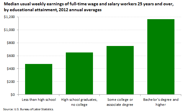
Educational Attainment | Median usual weekly earnings |
---|---|
Less than high school | $471 |
High school graduates, no college | 652 |
Some college or associate degree | 749 |
Bachelor's degree and higher | 1165 |
BLS publishes a large amount of workers' wages, earnings, and benefits data. Generally, these data focus on a geographic area (national, regional, state, metropolitan area, or county), occupation (for example, accountant, carpenter, or teacher), or industry (construction, manufacturing, retail trade, etc.). Data may also be available for age, sex, or union membership categories. This chart depicts median usual weekly earnings data by educational attainment.
While maxims about education and earnings may be clichés, they also may be true. In 2012, the median weekly earnings of full-time workers with bachelor's degrees or more education were $1,165. This amount is 1.8 times the median amount earned by those with only a high school diploma, and 2.5 times the earnings of high school dropouts.
Category | 2010 | 2011 | 2012 |
---|---|---|---|
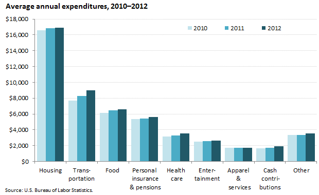
Housing | 16,557 | 16,803 | 16,887 |
Transportation | 7,677 | 8,293 | 8,998 |
Food | 6,129 | 6,458 | 6,599 |
Personal insurance and pensions | 5,373 | 5,424 | 5,591 |
Health care | 3,157 | 3,313 | 3,556 |
Entertainment | 2,504 | 2,572 | 2,605 |
Apparel and services | 1,700 | 1,740 | 1,736 |
Cash contributions | 1,633 | 1,721 | 1,913 |
Other | 3,379 | 3,382 | 3,557 |
The Consumer Expenditure (CE) Survey provides information on Americans' buying habits. CE data are used in a variety of research endeavors by government, business, labor, and academic analysts. The latest annual data show that in 2012 consumers increased spending in most of the seven major categories of expenditures tracked by CE: food, housing, transportation, healthcare, entertainment, and personal insurance and pensions. (Apparel and services is the lone exception). Gasoline expenditures (which are part of the transportation category) rose 29.6 percent from 2010 to 2012, but the majority of that was due to a 24.7 percent increase in 2011. In 2012 gasoline expenditures increased 4.0 percent.
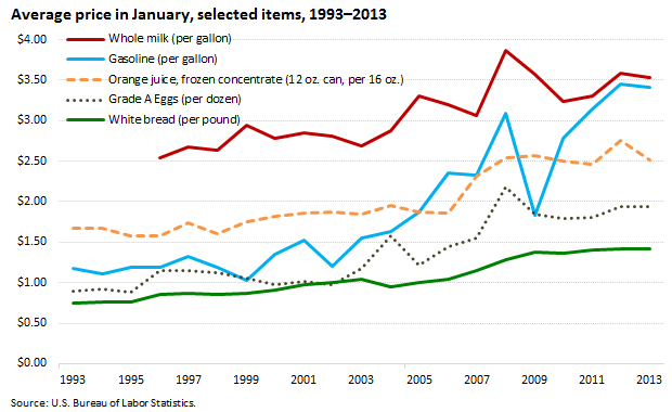
Year | Gasoline (per gallon) | White bread (per pound) | Grade A Eggs (per dozen) | Orange juice, frozen concentrate (12 oz. can, per 16 oz.) | Whole milk (per gallon) |
---|---|---|---|---|---|
1993 | 1.18 | 0.75 | 0.90 | 1.68 | (1) |
1994 | 1.11 | 0.77 | 0.92 | 1.67 | (1) |
1995 | 1.19 | 0.77 | 0.88 | 1.58 | (1) |
1996 | 1.19 | 0.86 | 1.16 | 1.58 | 2.55 |
1997 | 1.32 | 0.86 | 1.15 | 1.74 | 2.68 |
1998 | 1.19 | 0.86 | 1.12 | 1.60 | 2.63 |
1999 | 1.03 | 0.87 | 1.05 | 1.75 | 2.94 |
2000 | 1.36 | 0.91 | 0.98 | 1.82 | 2.79 |
2001 | 1.53 | 0.98 | 1.01 | 1.86 | 2.85 |
2002 | 1.21 | 1.00 | 0.97 | 1.88 | 2.81 |
2003 | 1.56 | 1.04 | 1.18 | 1.85 | 2.69 |
2004 | 1.64 | 0.95 | 1.57 | 1.96 | 2.88 |
2005 | 1.87 | 1.00 | 1.21 | 1.87 | 3.30 |
2006 | 2.36 | 1.05 | 1.45 | 1.85 | 3.20 |
2007 | 2.32 | 1.15 | 1.55 | 2.31 | 3.07 |
2008 | 3.10 | 1.28 | 2.18 | 2.54 | 3.87 |
2009 | 1.84 | 1.38 | 1.85 | 2.57 | 3.58 |
2010 | 2.78 | 1.36 | 1.79 | 2.50 | 3.24 |
2011 | 3.14 | 1.40 | 1.81 | 2.46 | 3.30 |
2012 | 3.45 | 1.42 | 1.94 | 2.75 | 3.58 |
2013 | 3.41 | 1.42 | 1.93 | 2.51 | 3.53 |
Footnotes:
(1) Not available.
|
A widely used measure of inflation, the Consumer Price Index (CPI) measures price movements for many goods and services. Each month, the CPI news release presents price changes for food, energy, housing, apparel, transportation, medical care, recreation, and education. The CPI shows how things like a drought in the Midwest, a freeze in the South, or a disruption in the supply of oil affect typical American consumers. The CPI is used to adjust wages and salaries for millions of workers and to keep pensions, rents, royalties, alimony, and child support payments in line with changing prices.
This chart shows average price data over the last twenty years for some common goods. Among the goods shown in the chart, gasoline prices have increased the most, from $1.18 a gallon in January 1993 to $3.41 a gallon in January 2013.
Year | Total | Age | Sex | Educational attainment (25 years and over) | |||
---|---|---|---|---|---|---|---|
16 years and over | 16 to 24 years | 25 years and over | Men | Women | High school graduates, no college | College graduates | |
2003 | 6.0 | 12.4 | 4.8 | 6.3 | 5.7 | 5.5 | 3.1 |
2004 | 5.5 | 11.8 | 4.4 | 5.6 | 5.4 | 5.0 | 2.7 |
2005 | 5.1 | 11.3 | 4.0 | 5.1 | 5.1 | 4.7 | 2.3 |
2006 | 4.6 | 10.5 | 3.6 | 4.6 | 4.6 | 4.3 | 2.0 |
2007 | 4.6 | 10.5 | 3.6 | 4.7 | 4.5 | 4.4 | 2.0 |
2008 | 5.8 | 12.8 | 4.6 | 6.1 | 5.4 | 5.7 | 2.6 |
2009 | 9.3 | 17.6 | 7.9 | 10.3 | 8.1 | 9.7 | 4.6 |
2010 | 9.6 | 18.4 | 8.2 | 10.5 | 8.6 | 10.3 | 4.7 |
2011 | 8.9 | 17.3 | 7.6 | 9.4 | 8.5 | 9.4 | 4.3 |
2012 | 8.1 | 16.2 | 6.8 | 8.2 | 7.9 | 8.3 | 4.0 |
The Current Population Survey (CPS) has been providing unemployment rates and other labor force data since the 1940s. Since that time, some observations about unemployment have remained true decade after decade. Persons age 16 to 24 years old typically have higher rates of unemployment than persons age 25 and over. Similarly, persons who only have a high school diploma are more likely to be unemployed than those with a bachelor’s degree or higher education.
During the recent recession (2007–2009), men’s unemployment rates tended to be higher than women’s. However, this has not been typical throughout the past eight decades of CPS unemployment data; before 1980, unemployment rates for women were typically higher then men’s.
To learn how unemployment estimates are calculated, please see How the Government Measures Unemployment.
Year | U-1 (Unemployed 15 Weeks & over) | U-2 (Job losers & persons who completed temporary jobs) | U-3 (Official unemployment rate) | U-4 (Unemployed & discouraged workers) | U-5 (Unemployed & marginally attached workers) | U-6 (Unemployed & marginally attached workers & part-time for economic reasons) |
---|---|---|---|---|---|---|
2003 | 2.3 | 3.3 | 6 | 6.3 | 7 | 10.1 |
2004 | 2.1 | 2.8 | 5.5 | 5.8 | 6.5 | 9.6 |
2005 | 1.8 | 2.5 | 5.1 | 5.4 | 6.1 | 8.9 |
2006 | 1.5 | 2.2 | 4.6 | 4.9 | 5.5 | 8.2 |
2007 | 1.5 | 2.3 | 4.6 | 4.9 | 5.5 | 8.3 |
2008 | 2.1 | 3.1 | 5.8 | 6.1 | 6.8 | 10.5 |
2009 | 4.7 | 5.9 | 9.3 | 9.7 | 10.5 | 16.2 |
2010 | 5.7 | 6 | 9.6 | 10.3 | 11.1 | 16.7 |
2011 | 5.3 | 5.3 | 8.9 | 9.5 | 10.4 | 15.9 |
2012 | 4.5 | 4.4 | 8.1 | 8.6 | 9.5 | 14.7 |
The official unemployment rate, which has been the standard way of measuring unemployment since the 1940s and which matches an international standard used by statistical agencies in other countries, is prominently featured in each month's Employment Situation news release. However, the BLS also publishes a set of alternative measures of labor underutilization known as U-1 through U-6 that are calculated with different definitions and are a help in understanding other labor market characteristics.
Unemployment as defined for U-1 includes only persons who have been unemployed for 15 weeks or longer. U-2 includes only job losers and persons who completed temporary jobs. Both U-1 and U-2 are lower than the official unemployment rate (known as U-3). The official unemployment rate (U-3) contains everyone included in U-1 and U-2 as well as all other persons who are not employed, are seeking employment, and are ready to work, regardless of how long they have been looking or their reason for unemployment.
U-4, U-5, and U-6 are higher than U-3 because they include additional persons who do not meet U-3’s definition of unemployment.
U-4 adds discouraged workers (persons with a job-market related reason for not currently looking for work).
U-5 adds persons marginally attached to the labor force (discouraged workers plus all other persons who are neither working nor currently looking for work but who indicate that they want and are available for a job and have looked for work sometime in the past 12 months).
U-6 builds on U-5 by adding persons who are employed part time for economic reasons—those who want and are available for full-time work but have had to settle for a part-time schedule.
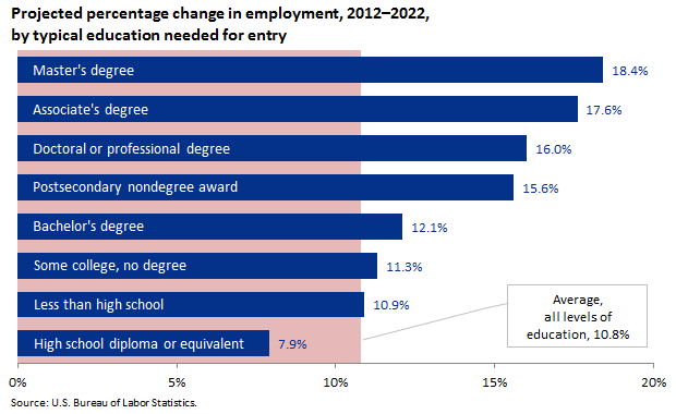
Education needed for entry | Percent change, projected 2012–2022 |
---|---|
Average, all occupations | 10.8% |
Master's degree | 18.4 |
Associate's degree | 17.6 |
Doctoral or professional degree | 16.0 |
Postsecondary nondegree award | 15.6 |
Bachelor's degree | 12.1 |
Some college, no degree | 11.3 |
Less than high school | 10.9 |
High school diploma or equivalent | 7.9 |
BLS projects occupational, industrial, and demographic trends into the future to give an idea how employment will change over the next several years. The Employment Projections office projects the fastest growing occupations, occupations with largest job growth, and the fastest growing and declining industries.
Occupations that typically require a master’s degree for entry are projected to grow the fastest during the 2012–2022 decade, followed by doctoral or professional degree, and associate’s degree occupations. All of the postsecondary groups are projected to grow faster than the average of 10.8 percent. The slowest growth is projected to be in occupations with high school diploma or equivalent as the typical entry-level education.
The Business Employment Dynamics program produces data that show job creation and destruction by size of establishment. (An establishment is a place of employment, such as a factory, office, or store.) During 2012, small establishments (those with fewer than 100 employees) created more jobs than the larger establishments (those with 100 or more employees). However, it is also true that more jobs were lost at the smaller establishments. These data show that as the size of establishment increases, the ratio of the number of jobs created to the number of jobs lost also increases. In other words, the difference between the number of jobs created and the number of jobs lost was larger among the larger establishments.
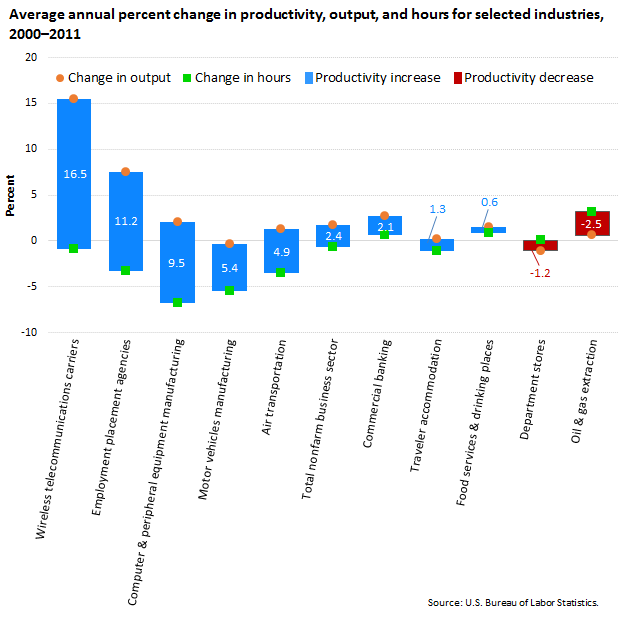
Industry | Productivity Growth | Change in output | Change in hours |
---|---|---|---|
Wireless telecommunications carriers | 16.5 | 15.4 | -0.9 |
Employment placement agencies | 11.2 | 7.6 | -3.3 |
Computer and peripheral equipment manufacturing | 9.5 | 2.0 | -6.8 |
Motor vehicles manufacturing | 5.4 | -0.3 | -5.4 |
Air transportation | 4.9 | 1.3 | -3.5 |
Total nonfarm business sector | 2.4 | 1.7 | -0.6 |
Commercial banking | 2.1 | 2.7 | 0.7 |
Traveler accommodation | 1.3 | 0.3 | -1.1 |
Food services and drinking places | 0.6 | 1.5 | 0.9 |
Department stores | -1.2 | -1.1 | 0.1 |
Oil and gas extraction | -2.5 | 0.6 | 3.2 |
Labor productivity, defined as output per hour of labor input, is a measure of how efficiently labor is used in the production of goods and services in the economy or in a particular industry. Increases in labor productivity are approximately equal to the difference between the growth of output and the growth of labor hours used to produce that output; the larger the gap between the growth of output and hours, the greater the productivity growth.
This chart shows output, hours, and labor productivity growth in the nonfarm business sector and in selected industries in that sector since 2000. During this period, productivity growth was particularly influenced by the growth of technology, the effects of business cycles, and increased globalization, to mention just a few factors. The wireless telecommunications industry maintained rapid output growth from 2000 to 2011 despite a slight decline in labor hours, a combination that reflected strong productivity growth. In contrast, most of the productivity growth in computer and peripheral equipment manufacturing was attributable to a much smaller increase in output and a large decline in hours. Productivity in the oil and gas extraction industry declined, as output growth did not keep pace with the growth in hours. Similarly, productivity declined in department stores, as output fell and labor hours were essentially unchanged.
Jan 1998 | 5,983,000 |
---|---|
Feb 1998 | 5,997,000 |
Mar 1998 | 5,969,000 |
Apr 1998 | 6,049,000 |
May 1998 | 6,087,000 |
Jun 1998 | 6,130,000 |
Jul 1998 | 6,172,000 |
Aug 1998 | 6,215,000 |
Sep 1998 | 6,225,000 |
Oct 1998 | 6,262,000 |
Nov 1998 | 6,301,000 |
Dec 1998 | 6,378,000 |
Jan 1999 | 6,357,000 |
Feb 1999 | 6,429,000 |
Mar 1999 | 6,402,000 |
Apr 1999 | 6,480,000 |
May 1999 | 6,516,000 |
Jun 1999 | 6,547,000 |
Jul 1999 | 6,571,000 |
Aug 1999 | 6,586,000 |
Sep 1999 | 6,613,000 |
Oct 1999 | 6,640,000 |
Nov 1999 | 6,687,000 |
Dec 1999 | 6,709,000 |
Jan 2000 | 6,752,000 |
Feb 2000 | 6,730,000 |
Mar 2000 | 6,811,000 |
Apr 2000 | 6,794,000 |
May 2000 | 6,770,000 |
Jun 2000 | 6,778,000 |
Jul 2000 | 6,794,000 |
Aug 2000 | 6,796,000 |
Sep 2000 | 6,807,000 |
Oct 2000 | 6,814,000 |
Nov 2000 | 6,817,000 |
Dec 2000 | 6,792,000 |
Jan 2001 | 6,824,000 |
Feb 2001 | 6,841,000 |
Mar 2001 | 6,862,000 |
Apr 2001 | 6,844,000 |
May 2001 | 6,849,000 |
Jun 2001 | 6,840,000 |
Jul 2001 | 6,845,000 |
Aug 2001 | 6,827,000 |
Sep 2001 | 6,813,000 |
Oct 2001 | 6,804,000 |
Nov 2001 | 6,784,000 |
Dec 2001 | 6,785,000 |
Jan 2002 | 6,775,000 |
Feb 2002 | 6,766,000 |
Mar 2002 | 6,755,000 |
Apr 2002 | 6,710,000 |
May 2002 | 6,684,000 |
Jun 2002 | 6,701,000 |
Jul 2002 | 6,688,000 |
Aug 2002 | 6,701,000 |
Sep 2002 | 6,702,000 |
Oct 2002 | 6,689,000 |
Nov 2002 | 6,713,000 |
Dec 2002 | 6,700,000 |
Jan 2003 | 6,704,000 |
Feb 2003 | 6,667,000 |
Mar 2003 | 6,654,000 |
Apr 2003 | 6,689,000 |
May 2003 | 6,706,000 |
Jun 2003 | 6,723,000 |
Jul 2003 | 6,735,000 |
Aug 2003 | 6,760,000 |
Sep 2003 | 6,783,000 |
Oct 2003 | 6,784,000 |
Nov 2003 | 6,796,000 |
Dec 2003 | 6,827,000 |
Jan 2004 | 6,848,000 |
Feb 2004 | 6,838,000 |
Mar 2004 | 6,887,000 |
Apr 2004 | 6,901,000 |
May 2004 | 6,948,000 |
Jun 2004 | 6,962,000 |
Jul 2004 | 6,977,000 |
Aug 2004 | 7,003,000 |
Sep 2004 | 7,029,000 |
Oct 2004 | 7,077,000 |
Nov 2004 | 7,091,000 |
Dec 2004 | 7,117,000 |
Jan 2005 | 7,095,000 |
Feb 2005 | 7,153,000 |
Mar 2005 | 7,181,000 |
Apr 2005 | 7,266,000 |
May 2005 | 7,294,000 |
Jun 2005 | 7,333,000 |
Jul 2005 | 7,353,000 |
Aug 2005 | 7,394,000 |
Sep 2005 | 7,415,000 |
Oct 2005 | 7,460,000 |
Nov 2005 | 7,524,000 |
Dec 2005 | 7,533,000 |
Jan 2006 | 7,601,000 |
Feb 2006 | 7,664,000 |
Mar 2006 | 7,689,000 |
Apr 2006 | 7,726,000 |
May 2006 | 7,713,000 |
Jun 2006 | 7,699,000 |
Jul 2006 | 7,712,000 |
Aug 2006 | 7,720,000 |
Sep 2006 | 7,718,000 |
Oct 2006 | 7,682,000 |
Nov 2006 | 7,666,000 |
Dec 2006 | 7,685,000 |
Jan 2007 | 7,725,000 |
Feb 2007 | 7,626,000 |
Mar 2007 | 7,706,000 |
Apr 2007 | 7,686,000 |
May 2007 | 7,673,000 |
Jun 2007 | 7,687,000 |
Jul 2007 | 7,660,000 |
Aug 2007 | 7,610,000 |
Sep 2007 | 7,577,000 |
Oct 2007 | 7,565,000 |
Nov 2007 | 7,523,000 |
Dec 2007 | 7,490,000 |
Jan 2008 | 7,476,000 |
Feb 2008 | 7,453,000 |
Mar 2008 | 7,406,000 |
Apr 2008 | 7,327,000 |
May 2008 | 7,274,000 |
Jun 2008 | 7,213,000 |
Jul 2008 | 7,160,000 |
Aug 2008 | 7,114,000 |
Sep 2008 | 7,044,000 |
Oct 2008 | 6,967,000 |
Nov 2008 | 6,813,000 |
Dec 2008 | 6,701,000 |
Jan 2009 | 6,554,000 |
Feb 2009 | 6,453,000 |
Mar 2009 | 6,291,000 |
Apr 2009 | 6,149,000 |
May 2009 | 6,103,000 |
Jun 2009 | 6,008,000 |
Jul 2009 | 5,928,000 |
Aug 2009 | 5,851,000 |
Sep 2009 | 5,785,000 |
Oct 2009 | 5,724,000 |
Nov 2009 | 5,693,000 |
Dec 2009 | 5,650,000 |
Jan 2010 | 5,581,000 |
Feb 2010 | 5,522,000 |
Mar 2010 | 5,542,000 |
Apr 2010 | 5,554,000 |
May 2010 | 5,527,000 |
Jun 2010 | 5,512,000 |
Jul 2010 | 5,497,000 |
Aug 2010 | 5,519,000 |
Sep 2010 | 5,499,000 |
Oct 2010 | 5,501,000 |
Nov 2010 | 5,497,000 |
Dec 2010 | 5,468,000 |
Jan 2011 | 5,435,000 |
Feb 2011 | 5,478,000 |
Mar 2011 | 5,485,000 |
Apr 2011 | 5,497,000 |
May 2011 | 5,524,000 |
Jun 2011 | 5,530,000 |
Jul 2011 | 5,547,000 |
Aug 2011 | 5,546,000 |
Sep 2011 | 5,583,000 |
Oct 2011 | 5,576,000 |
Nov 2011 | 5,577,000 |
Dec 2011 | 5,612,000 |
Jan 2012 | 5,629,000 |
Feb 2012 | 5,644,000 |
Mar 2012 | 5,640,000 |
Apr 2012 | 5,636,000 |
May 2012 | 5,615,000 |
Jun 2012 | 5,622,000 |
Jul 2012 | 5,627,000 |
Aug 2012 | 5,630,000 |
Sep 2012 | 5,633,000 |
Oct 2012 | 5,649,000 |
Nov 2012 | 5,673,000 |
Dec 2012 | 5,711,000 |
Jan 2013 | 5,735,000 |
Feb 2013 | 5,783,000 |
Mar 2013 | 5,799,000 |
Apr 2013 | 5,792,000 |
May 2013 | 5,791,000 |
Jun 2013 | 5,801,000 |
Jul 2013 | 5,804,000 |
Aug 2013 | 5,805,000 |
Current Employment Statistics estimates are calculated with data collected from employer payroll records. These monthly data show periods of employment contractions, recoveries, and expansions, which are the periods between peaks and troughs (maximum and minimum points, relative to each other).
A contraction in employment occurs when employment declines after a peak. The trough is reached when decreases stop and increases begin. The recovery is defined as a period of increasing employment from a trough until the employment level reaches the most recent peak. A period of continuing employment increases after the recovery is called an expansion, which leads to a new peak.
Note that the National Bureau of Economic Research, which publishes start and end dates for recessions in the United States, uses many types of data from various sources (not only employment data) to determine when recessions begin and end.
Month | Not seasonally adjusted | Seasonally adjusted |
---|---|---|
Jan 2008 | 15,458,300 | 15,570,300 |
Feb 2008 | 15,225,600 | 15,527,900 |
Mar 2008 | 15,279,000 | 15,506,200 |
Apr 2008 | 15,241,800 | 15,428,900 |
May 2008 | 15,296,300 | 15,379,300 |
Jun 2008 | 15,337,100 | 15,334,500 |
Jul 2008 | 15,302,400 | 15,298,800 |
Aug 2008 | 15,265,100 | 15,245,000 |
Sep 2008 | 15,093,800 | 15,172,000 |
Oct 2008 | 15,132,400 | 15,102,900 |
Nov 2008 | 15,346,000 | 14,980,700 |
Dec 2008 | 15,418,700 | 14,869,900 |
Jan 2009 | 14,682,700 | 14,784,300 |
Feb 2009 | 14,433,500 | 14,716,800 |
Mar 2009 | 14,404,800 | 14,620,900 |
Apr 2009 | 14,394,100 | 14,556,600 |
May 2009 | 14,490,000 | 14,553,500 |
Jun 2009 | 14,538,000 | 14,529,700 |
Jul 2009 | 14,483,600 | 14,485,200 |
Aug 2009 | 14,489,600 | 14,478,300 |
Sep 2009 | 14,362,000 | 14,436,000 |
Oct 2009 | 14,407,100 | 14,380,400 |
Nov 2009 | 14,724,200 | 14,370,800 |
Dec 2009 | 14,857,800 | 14,334,100 |
Jan 2010 | 14,285,000 | 14,384,700 |
Feb 2010 | 14,117,300 | 14,397,000 |
Mar 2010 | 14,203,500 | 14,420,500 |
Apr 2010 | 14,263,700 | 14,419,400 |
May 2010 | 14,374,500 | 14,434,400 |
Jun 2010 | 14,436,200 | 14,427,400 |
Jul 2010 | 14,439,500 | 14,442,600 |
Aug 2010 | 14,457,900 | 14,450,900 |
Sep 2010 | 14,355,200 | 14,470,700 |
Oct 2010 | 14,505,000 | 14,503,100 |
Nov 2010 | 14,844,200 | 14,486,000 |
Dec 2010 | 15,002,800 | 14,492,000 |
Jan 2011 | 14,443,100 | 14,547,200 |
Feb 2011 | 14,276,600 | 14,557,400 |
Mar 2011 | 14,343,300 | 14,564,200 |
Apr 2011 | 14,483,200 | 14,633,600 |
May 2011 | 14,582,900 | 14,638,700 |
Jun 2011 | 14,676,600 | 14,675,700 |
Jul 2011 | 14,712,000 | 14,709,800 |
Aug 2011 | 14,711,300 | 14,711,000 |
Sep 2011 | 14,611,700 | 14,732,800 |
Oct 2011 | 14,745,900 | 14,740,500 |
Nov 2011 | 15,136,500 | 14,769,000 |
Dec 2011 | 15,291,000 | 14,774,500 |
Jan 2012 | 14,728,900 | 14,829,000 |
Feb 2012 | 14,514,200 | 14,804,700 |
Mar 2012 | 14,574,400 | 14,799,100 |
Apr 2012 | 14,673,600 | 14,829,500 |
May 2012 | 14,787,300 | 14,838,900 |
Jun 2012 | 14,836,500 | 14,835,800 |
Jul 2012 | 14,838,500 | 14,838,900 |
Aug 2012 | 14,854,300 | 14,850,100 |
Sep 2012 | 14,786,500 | 14,876,200 |
Oct 2012 | 14,935,900 | 14,928,300 |
Nov 2012 | 15,430,300 | 14,997,900 |
Dec 2012 | 15,538,300 | 15,004,100 |
Jan 2013 | 14,944,000 | 15,026,500 |
Feb 2013 | 14,766,700 | 15,052,300 |
Mar 2013 | 14,815,700 | 15,049,500 |
Apr 2013 | 14,906,900 | 15,071,900 |
May 2013 | 15,029,700 | 15,104,500 |
Jun 2013 | 15,143,300 | 15,149,800 |
Jul 2013 | 15,192,400 | 15,190,800 |
Aug 2013 | 15,227,700 | 15,222,700 |
Sep 2013 | 15,147,000 | 15,243,500 |
When looking at unadjusted data, it is often difficult to tell whether changes from one month to another reflect changing economic conditions or only normal seasonal patterns that occur each year. These seasonal influences may result from seasonal climate conditions, manufacturing production cycles and model changeovers, and work, school, and holiday schedules. Many BLS data series are seasonally adjusted to remove the effect of seasonal influences.
In this chart of Current Employment Statistics employment estimates for the retail trade industry, the unadjusted data clearly show large increases at the end of each calendar year and corresponding decreases at the beginning of the next. During the recent recession (which began in December 2007 and ended in June 2009), even as employment was declining in most industries and the trend was down in retail trade, the seasonal increase and decrease still occurred. The seasonally adjusted data, from which the seasonal variation has been removed, more clearly shows the trend.
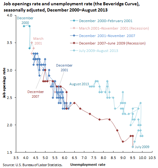
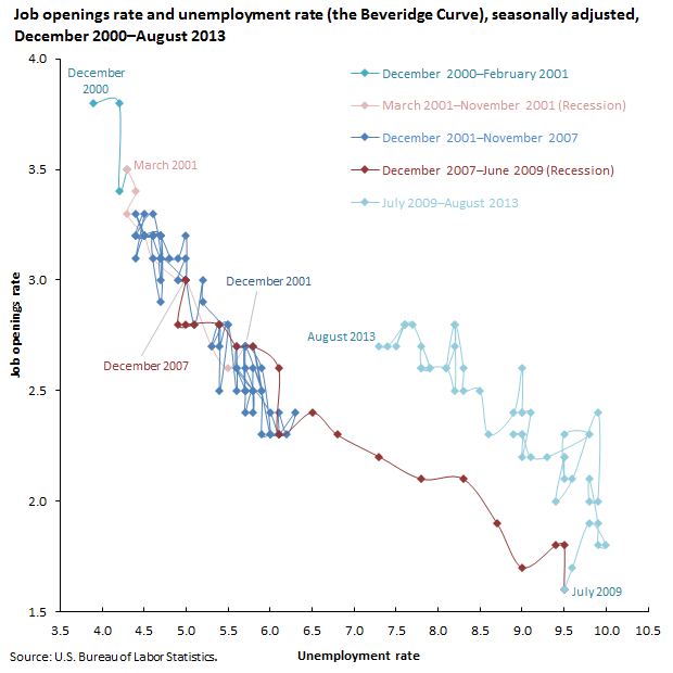
Month | Job openings rate | Unemployment rate |
---|---|---|
Dec 2000 | 3.8 | 3.9 |
Jan 2001 | 3.8 | 4.2 |
Feb 2001 | 3.4 | 4.2 |
Mar 2001 | 3.5 | 4.3 |
Apr 2001 | 3.4 | 4.4 |
May 2001 | 3.3 | 4.3 |
Jun 2001 | 3.2 | 4.5 |
Jul 2001 | 3.1 | 4.6 |
Aug 2001 | 3.0 | 4.9 |
Sep 2001 | 3.0 | 5.0 |
Oct 2001 | 2.7 | 5.3 |
Nov 2001 | 2.6 | 5.5 |
Dec 2001 | 2.7 | 5.7 |
Jan 2002 | 2.7 | 5.7 |
Feb 2002 | 2.5 | 5.7 |
Mar 2002 | 2.7 | 5.7 |
Apr 2002 | 2.5 | 5.9 |
May 2002 | 2.6 | 5.8 |
Jun 2002 | 2.4 | 5.8 |
Jul 2002 | 2.5 | 5.8 |
Aug 2002 | 2.6 | 5.7 |
Sep 2002 | 2.5 | 5.7 |
Oct 2002 | 2.7 | 5.7 |
Nov 2002 | 2.6 | 5.9 |
Dec 2002 | 2.3 | 6.0 |
Jan 2003 | 2.7 | 5.8 |
Feb 2003 | 2.5 | 5.9 |
Mar 2003 | 2.3 | 5.9 |
Apr 2003 | 2.3 | 6.0 |
May 2003 | 2.3 | 6.1 |
Jun 2003 | 2.4 | 6.3 |
Jul 2003 | 2.3 | 6.2 |
Aug 2003 | 2.4 | 6.1 |
Sep 2003 | 2.3 | 6.1 |
Oct 2003 | 2.4 | 6.0 |
Nov 2003 | 2.5 | 5.8 |
Dec 2003 | 2.4 | 5.7 |
Jan 2004 | 2.5 | 5.7 |
Feb 2004 | 2.6 | 5.6 |
Mar 2004 | 2.5 | 5.8 |
Apr 2004 | 2.6 | 5.6 |
May 2004 | 2.7 | 5.6 |
Jun 2004 | 2.5 | 5.6 |
Jul 2004 | 2.8 | 5.5 |
Aug 2004 | 2.7 | 5.4 |
Sep 2004 | 2.8 | 5.4 |
Oct 2004 | 2.8 | 5.5 |
Nov 2004 | 2.5 | 5.4 |
Dec 2004 | 2.8 | 5.4 |
Jan 2005 | 2.7 | 5.3 |
Feb 2005 | 2.8 | 5.4 |
Mar 2005 | 2.9 | 5.2 |
Apr 2005 | 3.0 | 5.2 |
May 2005 | 2.8 | 5.1 |
Jun 2005 | 3.0 | 5.0 |
Jul 2005 | 3.0 | 5.0 |
Aug 2005 | 3.0 | 4.9 |
Sep 2005 | 3.1 | 5.0 |
Oct 2005 | 3.0 | 5.0 |
Nov 2005 | 3.2 | 5.0 |
Dec 2005 | 3.1 | 4.9 |
Jan 2006 | 3.1 | 4.7 |
Feb 2006 | 3.1 | 4.8 |
Mar 2006 | 3.2 | 4.7 |
Apr 2006 | 3.2 | 4.7 |
May 2006 | 3.2 | 4.6 |
Jun 2006 | 3.1 | 4.6 |
Jul 2006 | 2.9 | 4.7 |
Aug 2006 | 3.2 | 4.7 |
Sep 2006 | 3.2 | 4.5 |
Oct 2006 | 3.1 | 4.4 |
Nov 2006 | 3.3 | 4.5 |
Dec 2006 | 3.2 | 4.4 |
Jan 2007 | 3.2 | 4.6 |
Feb 2007 | 3.2 | 4.5 |
Mar 2007 | 3.3 | 4.4 |
Apr 2007 | 3.2 | 4.5 |
May 2007 | 3.2 | 4.4 |
Jun 2007 | 3.3 | 4.6 |
Jul 2007 | 3.1 | 4.7 |
Aug 2007 | 3.2 | 4.6 |
Sep 2007 | 3.2 | 4.7 |
Oct 2007 | 3.0 | 4.7 |
Nov 2007 | 3.1 | 4.7 |
Dec 2007 | 3.0 | 5.0 |
Jan 2008 | 3.0 | 5.0 |
Feb 2008 | 2.8 | 4.9 |
Mar 2008 | 2.8 | 5.1 |
Apr 2008 | 2.8 | 5.0 |
May 2008 | 2.8 | 5.4 |
Jun 2008 | 2.7 | 5.6 |
Jul 2008 | 2.7 | 5.8 |
Aug 2008 | 2.6 | 6.1 |
Sep 2008 | 2.3 | 6.1 |
Oct 2008 | 2.4 | 6.5 |
Nov 2008 | 2.3 | 6.8 |
Dec 2008 | 2.2 | 7.3 |
Jan 2009 | 2.1 | 7.8 |
Feb 2009 | 2.1 | 8.3 |
Mar 2009 | 1.9 | 8.7 |
Apr 2009 | 1.7 | 9.0 |
May 2009 | 1.8 | 9.4 |
Jun 2009 | 1.8 | 9.5 |
Jul 2009 | 1.6 | 9.5 |
Aug 2009 | 1.7 | 9.6 |
Sep 2009 | 1.9 | 9.8 |
Oct 2009 | 1.8 | 10.0 |
Nov 2009 | 1.8 | 9.9 |
Dec 2009 | 1.9 | 9.9 |
Jan 2010 | 2.1 | 9.8 |
Feb 2010 | 2.0 | 9.8 |
Mar 2010 | 2.0 | 9.9 |
Apr 2010 | 2.4 | 9.9 |
May 2010 | 2.1 | 9.6 |
Jun 2010 | 2.0 | 9.4 |
Jul 2010 | 2.2 | 9.5 |
Aug 2010 | 2.2 | 9.5 |
Sep 2010 | 2.1 | 9.5 |
Oct 2010 | 2.3 | 9.5 |
Nov 2010 | 2.3 | 9.8 |
Dec 2010 | 2.2 | 9.3 |
Jan 2011 | 2.2 | 9.1 |
Feb 2011 | 2.3 | 9.0 |
Mar 2011 | 2.3 | 8.9 |
Apr 2011 | 2.3 | 9.0 |
May 2011 | 2.2 | 9.0 |
Jun 2011 | 2.4 | 9.1 |
Jul 2011 | 2.4 | 9.0 |
Aug 2011 | 2.4 | 9.0 |
Sep 2011 | 2.6 | 9.0 |
Oct 2011 | 2.4 | 8.9 |
Nov 2011 | 2.3 | 8.6 |
Dec 2011 | 2.5 | 8.5 |
Jan 2012 | 2.5 | 8.3 |
Feb 2012 | 2.6 | 8.3 |
Mar 2012 | 2.8 | 8.2 |
Apr 2012 | 2.6 | 8.1 |
May 2012 | 2.7 | 8.2 |
Jun 2012 | 2.8 | 8.2 |
Jul 2012 | 2.5 | 8.2 |
Aug 2012 | 2.6 | 8.1 |
Sep 2012 | 2.6 | 7.8 |
Oct 2012 | 2.6 | 7.9 |
Nov 2012 | 2.7 | 7.8 |
Dec 2012 | 2.6 | 7.8 |
Jan 2013 | 2.6 | 7.9 |
Feb 2013 | 2.8 | 7.7 |
Mar 2013 | 2.8 | 7.6 |
Apr 2013 | 2.7 | 7.5 |
May 2013 | 2.8 | 7.6 |
Jun 2013 | 2.8 | 7.6 |
Jul 2013 | 2.7 | 7.4 |
Aug 2013 | 2.7 | 7.3 |
A set of points, the position of each showing the unemployment rate for a given month plotted on one axis and the job openings rate for that month plotted on the other, forms a line known as the Beveridge Curve.* The Beveridge Curve slopes down from left to right, indicating that the job openings rate is high when the unemployment rate is low and vice-versa. During an economic slowdown or recession, as unemployment increases and the number of job openings decreases, the economy moves, month by month, lower and to the right along the curve. Economic growth during an expansion is seen as movement along the curve in the opposite direction, upwards and to the left.
December 2000 (on the Beveridge Curve for the December 2000–August 2013 period) is in the upper left corner of the chart, indicating a 3.8-percent job openings rate and a 3.9-percent unemployment rate. The points for March through November, a brief recession, are lower and to the right; during this period the job openings rate decreased from 3.5 percent to 2.6 percent, while the unemployment rate increased from 4.3 percent to 5.5 percent.
In the subsequent recovery and expansion period (December 2001–November 2007), the job openings rate ranged from 2.3 percent (during 2002 and 2003) to 3.3 percent (during 2006 and 2007) and unemployment rate ranged from 6.3 percent (during 2003) to 4.4 percent (2006 and 2007).
The recent recession saw the economy's position on the curve move significantly lower and to the right, from a point indicating a 3.0-percent job openings rate with a 5.0-percent unemployment rate (December 2007) to one showing a 1.8-percent job openings rate with a 9.5-percent unemployment rate (June 2009).
After the end of the recession, the job openings rate continued to decrease (reaching 1.6 percent in July 2009) and the unemployment rate continued to increase (reaching 10.0 percent in October 2009). Since that time, there have been improvements in both measures: higher job openings rates and lower unemployment rates.
* The unemployment rate comes from the Current Population Survey; the job openings rate from the Job Openings and Labor Turnover Survey. The Beveridge Curve is named for William Beveridge (1879–1963).
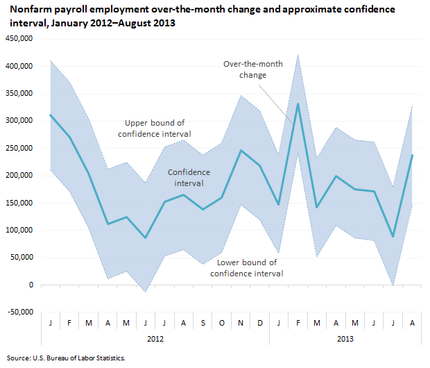
Month | Over-the-month change in nonfarm payroll employment | Lower bound of confidence interval | Upper bound of confidence interval |
---|---|---|---|
Jan 2012 | 311,000 | 211,000 | 411,000 |
Feb 2012 | 271,000 | 171,000 | 371,000 |
Mar 2012 | 205,000 | 105,000 | 305,000 |
Apr 2012 | 112,000 | 12,000 | 212,000 |
May 2012 | 125,000 | 25,000 | 225,000 |
Jun 2012 | 87,000 | -13,000 | 187,000 |
Jul 2012 | 153,000 | 53,000 | 253,000 |
Aug 2012 | 165,000 | 65,000 | 265,000 |
Sep 2012 | 138,000 | 38,000 | 238,000 |
Oct 2012 | 160,000 | 60,000 | 260,000 |
Nov 2012 | 247,000 | 147,000 | 347,000 |
Dec 2012 | 219,000 | 119,000 | 319,000 |
Jan 2013 | 148,000 | 58,000 | 238,000 |
Feb 2013 | 332,000 | 242,000 | 422,000 |
Mar 2013 | 142,000 | 52,000 | 232,000 |
Apr 2013 | 199,000 | 109,000 | 289,000 |
May 2013 | 176,000 | 86,000 | 266,000 |
Jun 2013 | 172,000 | 82,000 | 262,000 |
Jul 2013 | 89,000 | -1,000 | 179,000 |
Aug 2013 | 238,000 | 148,000 | 328,000 |
Note: The confidence interval was plus-or-minus 100,000 during 2012 and plus-or-minus 90,000 during 2013.
|
Statistical estimates based on a survey are subject to sampling error. When a sample (rather than the entire population) is surveyed, there is a chance that estimates calculated from the sample may differ from estimates calculated with data collected from the entire population. Statistical theory has shown that there is about a 90-percent chance (know as a level of confidence) that sampling error will cause an estimate based on a sample to differ by no more than 1.6 standard errors from the true population value which it estimates.
The confidence interval for the monthly change in total nonfarm employment from the Current Employment Statistics survey was on the order of plus or minus 100,000 during 2012. In June 2012, the estimate of the change in nonfarm employment (87,000) was less than 100,000. The 90-percent confidence interval for that month's change would range from 187,000 (which is 87,000 plus 100,000) to -13,000 (87,000 - 100,000). These figures do not mean that the sample results are off by these amounts, but rather that there is about a 90-percent chance that the actual over-the-month change lies within this interval. Because this range includes values of less than zero, we can not say with confidence that nonfarm employment had, in fact, increased that month. It was the same story in July 2013, when the estimate was 89,000 and the confidence interval was plus or minus 90,000.
Consider, however, the reported nonfarm employment increases in all of the other months since January 2012; for example, the increase of 148,000 in January 2013. All of the values within the 90-percent confidence interval are greater than zero, and thus it is likely (there is at least a 90-percent chance) that nonfarm employment did, in fact, rise that month.
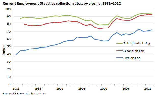
Year | First closing | Second closing | Third (final) closing |
---|---|---|---|
1981 | 39.6 | ||
1982 | 44.6 | 87.1 | |
1983 | 45.0 | 79.9 | 89.2 |
1984 | 46.8 | 78.1 | 88.3 |
1985 | 47.3 | 77.8 | 88.1 |
1986 | 47.9 | 78.0 | 87.3 |
1987 | 48.9 | 78.7 | 87.8 |
1988 | 49.4 | 80.5 | 89.0 |
1989 | 51.3 | 81.5 | 89.8 |
1990 | 52.2 | 82.1 | 90.8 |
1991 | 54.0 | 82.0 | 90.3 |
1992 | 56.8 | 83.2 | 91.1 |
1993 | 57.9 | 84.2 | 91.6 |
1994 | 58.0 | 83.1 | 90.3 |
1995 | 62.6 | 83.1 | 89.1 |
1996 | 62.1 | 80.3 | 86.7 |
1997 | 61.8 | 78.3 | 84.1 |
1998 | 64.1 | 79.8 | 85.1 |
1999 | 59.2 | 75.6 | 80.9 |
2000 | 58.6 | 74.0 | 78.9 |
2001 | 57.4 | 74.7 | 79.2 |
2002 | 57.8 | 74.7 | 79.0 |
2003 | 65.0 | 82.6 | 85.7 |
2004 | 68.9 | 87.2 | 90.9 |
2005 | 64.9 | 85.4 | 88.5 |
2006 | 66.9 | 85.0 | 87.7 |
2007 | 65.9 | 84.9 | 87.4 |
2008 | 68.6 | 87.6 | 90.9 |
2009 | 73.3 | 90.5 | 93.1 |
2010 | 70.4 | 91.6 | 94.3 |
2011 | 71.1 | 92.7 | 94.1 |
2012 | 72.5 | 92.6 | 94.6 |
The accuracy of BLS estimates results directly from the participation of the many households and businesses establishments that provide their data in BLS surveys. An accurate estimate of U.S. employment would be impossible without the employers that participate in the Current Employment Statistics (CES) payroll survey.
There are three collection deadlines or "closing dates" in the CES data collection process, the first during the reference month, the second and third in the two subsequent months. In 2012, the average collection rate was 73.1 percent for the first closing date and 94.6 percent for the third and final closing date. This is the highest annual average for the 21-year period for which these data have been maintained and an overall improvement over the previous two decades when rates were in the 80 to 90 percent range.
To learn more about the CES collection and revision process, see "Why are there revisions to the jobs numbers?" (Beyond the Numbers, July 2013).
These BLS Overviews and publications are guides for more statistical explorations.
BLS Overviews |
BLS Publications
International Year of Statistics—Statistics2013The founding organizations of the International Year of Statistics—also called Statistics2013—are the American Statistical Association, Institute of Mathematical Statistics, International Biometric Society, International Statistical Institute (and the Bernoulli Society), and Royal Statistical Society. |