
An official website of the United States government
An official website of the United States government
The .gov means it's official.
Federal government websites often end in .gov or .mil. Before sharing sensitive information,
make sure you're on a federal government site.
The site is secure.
The
https:// ensures that you are connecting to the official website and that any
information you provide is encrypted and transmitted securely.
Robert S. Martin, Brett Matsumoto, Thesia I. Garner, Scott Curtin
December 9, 2024
We estimate group-specific personal consumption expenditure (PCE) price indexes for 2000-2022 for deciles of equivalized PCE. To do this, we aggregate detailed category PCE price indexes from National Income and Product Account (NIPA) Table 2.4.4U using weights which vary by group for 150 detailed spending categories. Group weights based on equivalized PCE are estimated using the distributional PCE methods described in Garner, et al. (2022, 2024).
We generally find a negative relationship between PCE inflation and expenditure, similar to the recent literature on consumer price indexes by income. Grouping households by equivalized PCE, the first decile of equivalized PCE had average annual inflation that was 0.32 percentage points higher than the ninth decile and 0.18 percentage points higher than the official PCE price index for the 2000-2022 period. Average inflation for the tenth decile, however, was only 0.13 percentage points lower than that of the first decile. Restricting the index to market-based PCE, the relationship between average inflation and expenditure was monotonic, with the bottom decile exceeding the top decile by 0.48 percentage points per year. Market-based PCE excludes categories such as imputed financial services which are not included in the U.S. consumer price index (CPI) nor measured by the Consumer Expenditure Surveys (CE). These categories are not paid for out-of-pocket by households, are concentrated at the top of the spending distribution, and have high inflation over the study period. The market-based PCE patterns and magnitude are similar to results from Klick and Stockburger (2024) for equivalized income groupings.[1]
Heterogenous PCE price inflation has implications for changes in real inequality over this period. Accounting for differential inflation, the proportional gap between the first and tenth deciles of the equivalized PCE distribution widened rather than shrunk over this period.
Our strategy for estimating distributional price indexes is to re-weight the detailed PCE price subindexes from NIPA table 2.4.4U using group-specific expenditure shares, similar to the exercises in Klick and Stockburger (2024) and Jaravel (2024). All results in this report are based on PCE data released on September 26, 2024. Using weights from the current and prior year, the BEA uses a chained Fisher formula to aggregate basic indexes, most of which are CPIs or producer price indexes (PPI) produced by the Bureau of Labor Statistics (BLS).[2] The Fisher index is the geometric average of the Laspeyres and Paasche indexes. The group-specific expenditure shares are based on distributional PCE estimates. More detailed descriptions of the distributional PCE methodology can be found in Garner, et al. (2022, 2024).
Mathematically, let the decile d specific expenditure share for PCE category a in year t be defined as:
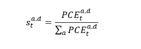
Where is the PCE expenditures for category for decile. If PCEPI is the PCE price index, then the PCE decile specific inflation is given by:
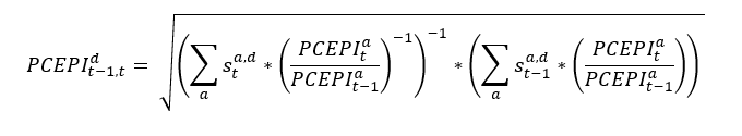
The first term under the square root is the Paasche index and the second term is the Laspeyres index. It is important to note that in this exercise, the category level inflation is the same for all groups. Differences in inflation between groups comes from differences in the expenditure shares.
The distributional PCE methodology can be briefly summarized as follows. We first map CE product categories to their closest PCE counterparts. We then statistically match CE Diary observations to CE Interview observations to cover about 6% of eligible expenditures not available in the Interview[3]. We then make several imputations for categories which are out-of-scope for CE, including third-party health care expenditures. We restrict our CE sample to consumer units with at least two interviews and annualize their expenditures. We also apply a top tail adjustment based on the Pareto distribution to the top 5% of total spending to mitigate potential understatement of inequality. We then scale CE spending to match PCE aggregates for various categories. Finally, all quantile groupings are based on adult-equivalized PCE using the square root of family-size.
This yields expenditure group-specific spending estimates for 150 categories which scale to PCE aggregates. These 150 categories cover the breadth of the 244 most detailed categories from NIPA Table 2.4.5U, but we are not always able match CE and PCE at the most detailed level. Some detailed categories have no counterpart in the CE (e.g., 22 categories for non-profit institutions serving households), and some are either more disaggregated in PCE (e.g., foreign vs domestic autos) or have spotty coverage in the CE due to sample size (e.g., pleasure aircraft). In these cases, to take new automobiles as an example, our price indexes reflect differences across groups in spending shares on new automobiles out of all goods and services, but not spending share differences on foreign vs. domestic automobiles.
Finally, we present indexes for expenditure groups over time as if membership is static, similar to Klick and Stockburger (2024) and Jaravel (2024). As such, long-run inflation estimates for a particular quantile should be interpreted somewhat cautiously, as in reality a specific household may move within the expenditure distribution over time.
For the study period, we find a nonmonotonic relationship between PCE inflation and expenditure level. From Figure 1, average annual inflation falls by decile from 2.26% for the first decile to 1.94% for the ninth decile, but then rises 0.19 percentage points between the ninth and tenth deciles. For market-based PCE (Figure 2), the relationship is negative and monotonic, with the first decile averaging about 0.48 percentage points higher inflation per year than the tenth decile. Table 3 of the PCE distributional results file for 2000-2022 has the full index results by decile of equivalized PCE.
The non-monotonic pattern of inflation by decile for PCE is worth further examination, given that this departs from the monotonic decreasing pattern observed in the literature and with market-based PCE. Figure 3 compares total and market-based PCE by decile of total equivalized PCE for 2017 (chosen because 2017 is BEA’s base year for the published PCE price indexes, for which they equal 100). Overall, market-based PCE comprises about 87% of total PCE, though by decile this varies from about 81% for the top decile to 92% for the bottom decile. According to the BEA, the market-based PCE “excludes most imputed expenditures such as ‘financial services furnished without payment’”, but it does include imputed rent for owner-occupied housing, making the index more comparable to the CPI and CE Program CE-PCE comparison.
Figure 4 shows how the non-market expenditures are distributed by category for each decile. In particular, financial services and insurance make up over 40% of non-market PCE overall and over 60% for the top decile. At the same time, these expenditures include categories which had much higher inflation than average over our study period.
Figure 5 compares levels for the overall PCE price index, the subindex for financial services and insurance. Within financial services, we also plot the indexes for financial services furnished without payment and portfolio management and investment advice services. Over this period, cumulative inflation for financial services and insurance was 35 percentage points higher than overall PCE, financial services furnished without payment was 74 percentage points higher than overall PCE, and portfolio management and investment advice services was 121 percentage points higher than overall PCE. Non-market spending on financial services and insurance were also concentrated at the top of the total spending distribution—the top decile had 46% of non-market financial services and insurance in 2017, for instance. These aggregates are imputed, as they do not reflect explicit charges to households. They are not included in the U.S. CPI, and BEA uses PPIs for related services as the deflators.
Most non-market PCE concepts also must be imputed in the micro data for distributional analysis. For instance, we allocate financial services furnished without payment from commercial banks and other depository institutions to be proportional to the values of financial asset holdings.[4] As a result, distributional results pertaining to non-market expenditures may be subject to a larger degree of error than market-based expenditures.
Finally, the inflation differences we find are meaningful for measures of real growth. To illustrate, Figure 6 compares cumulative growth in real PCE from 2000-2022 across deciles using both the official PCE price index to deflate each decile’s spending or using the price indexes specific to each decile. Using the official deflator, the gap in real PCE between the tenth and first decile narrowed by 0.6% ((1.67/1.68 – 1)*100%), while the gap between the ninth and first decile narrowed by 2.8% ((1.63/1.68 – 1)*100%). Using the distributional PCE price indexes, the 10-to-1 gap widened by 2.1%, and the 9-to-1 gap widened by 4.1%. The impact on relative growth in real market-based PCE (Figure 7) are larger. Using the official deflator, the 10-to-1 gap narrowed by 1.3%, while using the distributional deflators, the gap widened by 9.3%.
In line with the recent literature on CPI inflation across the income distribution, we find substantial differences in price change across the expenditure distribution when using the PCE concept. One implication for inequality measurement is that accounting for inflation differences leads to smaller narrowing of the gap between real PCE at the top and bottom of the expenditure distribution. The nonmonotonic relationship between expenditure and PCE inflation appears specific to the PCE concept (as opposed to distributional CPIs) because it includes non-market spending which is usually excluded from a CPI. As this spending is imputed in both the macro and micro data, its impact on the distributional results should be interpreted somewhat cautiously. The concentration of these non-market expenditures at the top of the PCE distribution underscores the need to account for detailed spending pattern differences.
Garner, Thesia I., Robert S. Martin, Brett Matsumoto, and Scott Curtin. 2022. Distribution of U.S. Personal Consumption Expenditures for 2019: A Prototype Based on Consumer Expenditure Survey Data. Working Paper 557, Washington DC: Bureau of Labor Statistics. https://www.bls.gov/osmr/research-papers/2022/pdf/ec220120.pdf.
Garner, Thesia I., Robert S. Martin, Brett Matsumoto, and Scott Curtin. 2024. Distribution of U.S. Personal Consumption Expenditures Using Consumer Expenditure Survey Data: Methodology Update and Supplementary Results. Washington, D.C.: U.S. Bureau of Labor Statistics. https://www.bls.gov/cex/pce-ce-distribution-methods.htm.
Jaravel, Xavier. 2024. "Distributional Consumer Price Indexes." Working paper. https://www.xavierjaravel.com/_files/ugd/bacd2d_1bd06a592911439a9f9c8a1ddfe6f6df.pdf.
Jaravel, Xavier. 2019. "The Unequal Gains from Product Innovations: Evidence from the U.S. Retail Sector." The Quarterly Journal of Economics 715-783. doi:doi.org/10.1093/qje/qjy031.
Klick, Joshua, and Anya Stockburger. 2024. "Examining U.S. inflation across households grouped by equivalized income." Monthly Labor Review (July 2024). doi:10.21916/mlr.2024.12.
U.S. Bureau of Economic Analysis. 2023. "Chapter 4: Estimating Methods." In Handbook of Methods, by U.S. Bureau of Economic Analysis, 1-30. Washington DC: U.S. Bureau of Economic Analysis. https://www.bea.gov/resources/methodologies/nipa-handbook/pdf/chapter-04.pdf.
U.S. Bureau of Economic Analysis. 2023. "Chapter 5: Personal Consumption Expenditures." In Handbook of Methods, by Bureau of Economic Analysis, 1-69. Washington, DC: Bureau of Economic Analysis. https://www.bea.gov/resources/methodologies/nipa-handbook/pdf/chapter-05.pdf.
[1] For 2006-2022, Klick and Stockburger (2024) find the bottom quintile of equivalized income had 0.41 percentage points per year higher inflation than the top quintile using formulas similar the Tornqvist Chained CPI-U. Figure 2 of Jaravel (2024), using public-use CE and CPI data for 2002-2024, also shows a similar gap between the top and bottom 5% of income.
[2] See https://www.bea.gov/resources/methodologies/nipa-handbook/pdf/chapter-04.pdf.
[3] This figure comes after mapping CE to PCE categories, but prior to any imputations and adjustments to close the micro-macro gap.
[4] Additionally, the CE only collects information on assets and liabilities in the fourth interview, which not all households in our sample complete. We therefore impute missing observations using a statistical matching algorithm based on income, age of the reference person, and race of the reference person.
Last Modified Date: December 9, 2024