An official website of the United States government
 United States Department of Labor
Aaron Cobet
Bureau of Labor Statistics
February 3, 2017
The Consumer Expenditure Surveys Program (CE) collects data on all reported expenditures and most types of income in the United States. CE provides these data by geographic region and many demographic characteristics.
However, some CE estimates may not be precise enough for your needs because CE may only provide a wide range of possible values rather than an exact data point.1 This report addresses these related questions:
Data that are based on surveys have some degree of variability, which means that the reported value is an approximation of the actual value. Generally, the reported value is an average of the sampled observations. The size of the variability dependds on two factors.
| 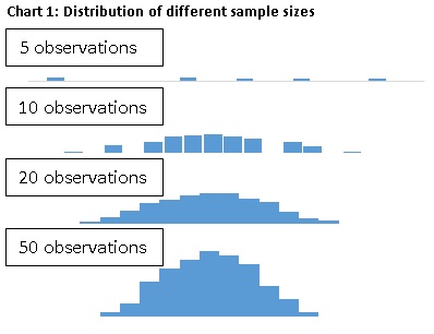 |
| 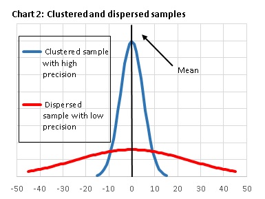 |
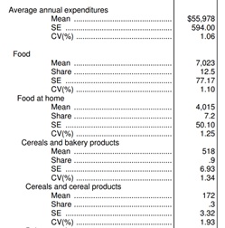
The CE tables provide two measures of variability:
A SE measures the absolute dispersion of an estimate. For CE, SE shows how close the dollar average of the sample is to the average of the populations. CE calculates a modified version of the standard SE formula due to its sample design.2
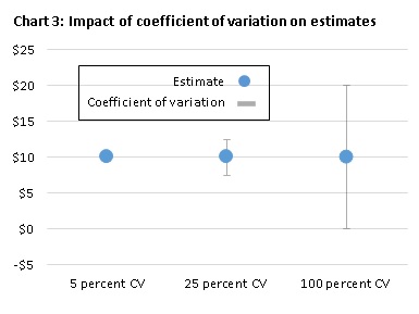
Variability limits your ability to use the data with certainty. Measures of variability inform you about the range of possible values for a particular data point. Generally, the larger that range is the lower your confidence in the data point.3
Chart 3 shows the effect of increasing ranges on the range of possible values with three different CVs:
The range of the possible estimates expands with a 5 percent CV to values between $9.50 and $10.50, with a 25 percent CV to $12.50 to $7.50, and with a 100 percent CV to $0.00 and $20.00. The third example shows how a large CV may affect your analysis.
The CE tables show the degree of precision with CVs. CE staff strongly recommend using estimates with CVs that are below 25 percent. CV's of 25 percent allow you to state with certainty that the actual value is no larger or smaller than 25 percent of the estimate.4 However, there is no rule about what precision is sufficient for your analysis. For more information on this topic, see when can you compare two data points with confidence?
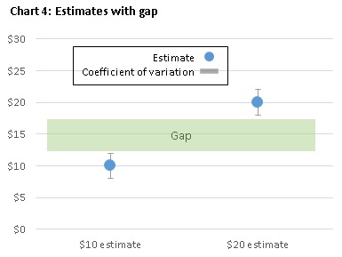
You can determine which data point is larger if there is a gap between two points after you consider their variation or CV. By contrast you cannot determine which estimate is larger if the two data points with their CVs overlap.
Charts 4 and 5 provide examples for both scenarios. Both charts show on the left a $10 estimate and on the right a $20 estimate.
In chart 4, the two estimates have a gap after taking their CV into account. In this case, you can determine that the $10 estimate is definitively smaller than the $20 estimate because the biggest possible value of the $10 estimate is $12.50 and the smallest possible value of the $20 estimate is to $17.50. Since $12.50 is smaller than $17.50, the $10 estimate is smaller than the $20 estimate.
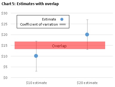
In contrast, chart 5 shows two data points that have an overlap after taking their CV into account. In this case, you cannot determine with certainty that the $10 estimate is smaller than the $20 estimate because the biggest possible value of the $10 estimate is $17, and the smallest possible value of the $20 estimate is $13. Since $17 is larger than $13, the $10 estimate might be larger than the $20 estimate.
You can increase the precision of estimates or decrease its range of possible values by increasing the number of observations in your sample. You can increase the sample size by expanding your research question and dropping aspects from consideration that are less important to your analysis.
Let's say you want to look at expenses for men's shirts in the Northeast by households earning $50,000 to $69,999 in 2015. However, you determine that the data are not precise enough for your analysis. You could drop the least important aspect until the precision meets your needs.
For CE data, you may be able to increase your sample with these changes:
You can use these methods to a varying degree with two CE products:
For additional information on this issue, CE provides these resources:
1 CE data can be used to derive two types of estimates. CE tables and the database provide weighted population estimates, which refer to estimates that have been weighted to be representative of the entire population. In addition, users can use Public-use Microdata to calculate not only other weighted population estimates, but also unweighted sample estimates, which provide an estimate for the respondents who made this expenditure or had this income type.
2 CE does not calculate the standard error with the standard formula because this formula requires that the sample is collected as a simple random sample. However, the CE surveys draw stratified random samples of geographic areas and a systematic sample of households within the selected areas. To estimate an unbiased variance with this sampling method, CE uses the balanced repeated replication (BRR) method. For more information on this issue, see "Standard Errors in the 2015 Consumer Expenditure Survey".
3 This range is called confidence interval, which measures the probability that a population parameter falls between two values.
4 CE estimates do not provide 100 percent certainty. For more information on the degree of certainty of CE estimates, see Standard Errors in the 2015 Consumer Expenditure Survey by David Swanson.
Last Modified Date: February 3, 2017