An official website of the United States government
An official website of the United States government
The .gov means it's official.
Federal government websites often end in .gov or .mil. Before sharing sensitive information,
make sure you're on a federal government site.
The site is secure.
The
https:// ensures that you are connecting to the official website and that any
information you provide is encrypted and transmitted securely.
April 2011
Montana employed bartenders at 3 times the national rate in May 2009, Delaware employed chemists at nearly 8 times the national rate, fast food cooks were 3 times as concentrated in Mississippi as in other parts of the country, and computer software engineers were more than twice as prevalent in Virginia as elsewhere. These comparisons are easily made through the use of location quotients.
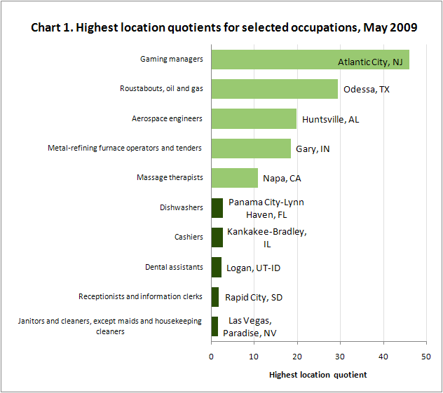
Some familiar and some not-so-familiar patterns emerge when looking at location quotient data. For example, the areas with the highest location quotients for several gaming occupations included Atlantic City and several areas in Nevada. Atlantic City and Las Vegas also had among the highest concentrations of bartenders, as did areas in the northern states of Montana, Wisconsin, North Dakota, and Minnesota. Areas that tend to be tourist destinations had higher location quotients for leisure-related occupations, such as high concentrations of restaurant cooks in Nantucket and Martha’s Vineyard and massage therapists in Napa, CA. Palm Bay-Melbourne-Titusville, FL, the home of Kennedy Space Center, had one of the highest location quotients for aerospace engineers, while areas in Michigan, Indiana, and Ohio had high location quotients for several production occupations.
Location quotients are useful for studying the composition of jobs in an area relative to the average, or for finding areas that have high concentrations of jobs in certain occupations. As measured here, a location quotient shows the occupation’s share of an area’s employment relative to the national average. For example, a location quotient of 2.0 indicates that an occupation accounts for twice the share of employment in the area than it does nationally, and a location quotient of 0.5 indicates the area’s share of employment in the occupation is half the national share. For instance, home health aides accounted for nearly 2 percent of employment in North Carolina in May 2009, but less than 1 percent of employment in the United States, giving the occupation a location quotient of more than 2 in North Carolina.
Location quotients show how occupations are spread out across the country. The location quotients for some occupations clustered around 1.0, indicating that they were found in similar proportions in most areas. For example, the location quotients for janitors ranged from 0.5 to 1.6, and those for receptionists and information clerks ranged from 0.5 to 1.7. (Chart 1.) Other occupations with relatively even geographic distributions included dental assistants, cashiers, and dishwashers.
Other occupations were more concentrated and had very high location quotients in some areas. These were often occupations directly related to industries that are geographically concentrated. For example, the employment share of textile knitting and weaving machine setters, operators, and tenders in Dalton, GA, was nearly 197 times the national average; this area also had high location quotients for several other textile and apparel production occupations, as did other southern areas such as Hickory-Lenoir-Morganton, NC; Anderson, SC; and Greensboro-High Point, NC.
Some of the occupations with the highest location quotients were associated with geographical features such as waterways or natural resource deposits. For example, Houma-Bayou Cane-Thibodaux, LA, had very high location quotients for several water transportation occupations, including ship engineers, with a location quotient of 91; sailors and marine oilers, with a location quotient of 114; and captains, mates, and pilots of water vessels, with a location quotient of 150. Similarly, occupations associated with mining or oil and gas extraction tended to have very high location quotients in some areas. Charleston, WV, had location quotients of 52 for minecutting and channeling machine operators and 66 for mining roof bolters, while Odessa, TX, had high concentrations of several oil-related occupations, including location quotients of 29 and 58, respectively, for roustabouts and oil, gas, and mining service unit operators.
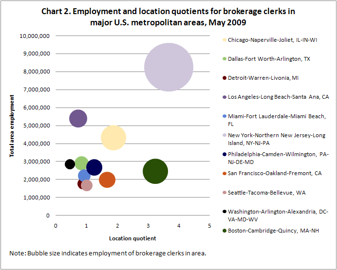
In some cases, more complex patterns emerge. Chart 2 shows employment and location quotients for brokerage clerks in the largest metropolitan areas in the United States. In general, areas with higher employment of brokerage clerks also had higher location quotients for this occupation, suggesting that there is some advantage to having large numbers of workers in this financial services occupation clustered together. Because the location quotients control for area size, we might expect that an occupation’s employment would not be correlated with the size of the area. However, although the relationship was not extremely strong, brokerage clerks also were somewhat more likely to be employed in areas with higher overall employment.
Some occupations had higher location quotients in smaller areas, such as purchasing agents and buyers of farm products, which were somewhat more likely to be concentrated in areas with low total employment. In this case, there was no correlation between an area’s location quotient and employment of this specific occupation: because areas with low overall employment also tend to have low employment of most individual occupations, many of the areas with high concentrations of purchasing agents and buyers of farm products had relatively low employment levels for this occupation. For example, Sioux City, IA-NE-SD, had an employment concentration of nearly 8 times the U.S. average for purchasing agents and buyers of farm products, but had employment of only 50 in this occupation. In contrast, the much larger New York-Northern New Jersey-Long Island, NY-NJ-PA, metropolitan area employed over 500 purchasing agents and buyers of farm products, but had a location quotient of 0.7 for this occupation.
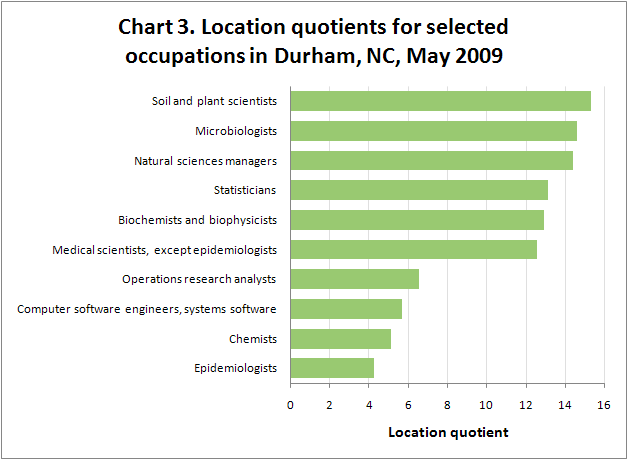
A closer look at two areas—Durham, NC, and Columbus, IN—is provided in charts 3 and 4. Durham, in the heart of North Carolina’s Research Triangle, had high location quotients for several life science occupations, including soil and plant scientists, microbiologists, biochemists and biophysicists, medical scientists, and epidemiologists. This area also had high concentrations of other occupations associated with scientific research, including natural sciences managers and statisticians, as well as computer systems software engineers and several other computer occupations not shown in the chart.
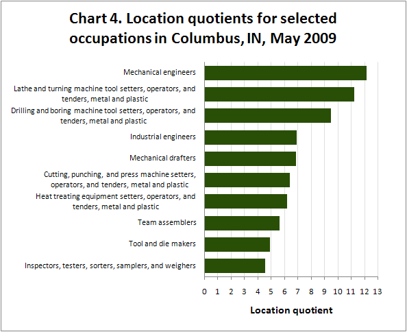
Columbus, IN, had high location quotients for a number of production occupations, including team assemblers; tool and die makers; inspectors, testers, sorters, samplers, and weighers; and several metal and plastic worker occupations. In addition, this area had high concentrations of several occupations associated with the design and engineering stages of the manufacturing process: the concentration of mechanical engineers was over 12 times the U.S. average, while both industrial engineers and mechanical drafters had concentrations nearly 7 times the U.S. average.
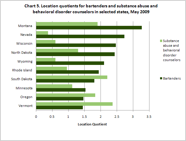
Chart 5 shows location quotients for bartenders and substance abuse and behavioral disorder counselors in various states. As mentioned above, Montana had the highest location quotient for bartenders, at 3.3 times the national average. Montana also had the fourth highest location quotient for substance abuse and behavioral disorder counselors. Several other states had location quotients in the top 10 for both bartenders and substance abuse and behavioral disorder counselors, including South Dakota, Oregon, and Vermont. However, there are exceptions, such as Nevada, where the location quotient for substance abuse and behavioral disorder counselors was smaller than every other state except West Virginia at 0.37.
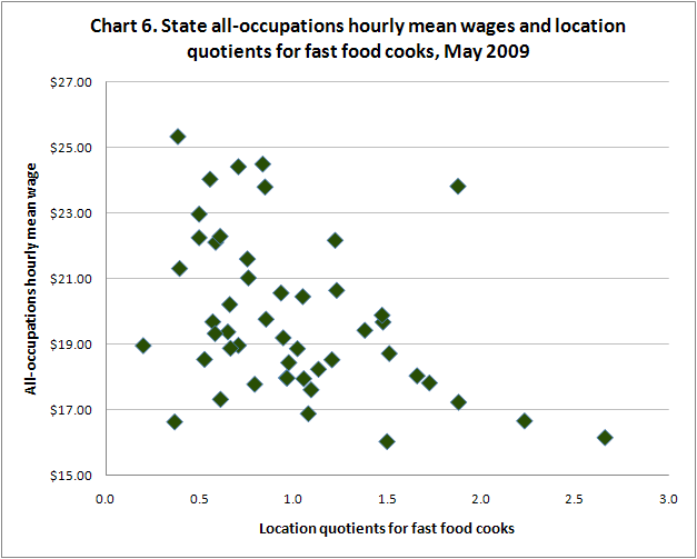
Location quotients can also help explain wage differences among areas. The composition of employment in an area influences the average wage in that area. All else equal, areas with higher employment shares of lower paid occupations such as fast food cooks and cashiers will tend to have lower average wages, in part because the concentration of employment in these occupations helps bring down the average area wage. The correlation coefficient on the share of fast food cooks in a state and the state’s cross-occupation wage was -.44, indicating that, generally, areas with higher concentrations of fast food cooks had lower average wages. (See chart 6.)
Areas with greater concentrations of higher paying occupations such as financial managers and biochemists and biophysicists tended to have higher cross-occupation wages. For example, states with high shares of business and financial operations occupations and computer and mathematical science occupations also tended to have higher wages: average cross-occupation wages and employment shares in these occupations were correlated with coefficients of 0.85 and 0.76, respectively. Other occupations that tended to be more concentrated in higher wage areas were arts, design, entertainment, sports, and media occupations.
The location quotients used in this highlight were calculated from May 2009 Occupational Employment Statistics; location quotients for all occupations and areas are available at https://www.bls.gov/oes/special-requests/oesm09ma.zip. Complete May 2009 OES data are available from the OES home page at https://www.bls.gov/oes. This highlight was prepared by Ben Cover. For more information, please contact the OES program at https://www.bls.gov/oes/oes_con.htm.
Last Modified Date: March 30, 2018