The Challenges of Seasonal Adjustment during the COVID-19 Pandemic

In a previous edition of Commissioner’s Corner, we described seasonal adjustment, the process BLS and many others use to smooth out increases and decreases in data series that occur around the same time each year. Seasonal adjustment allows us to focus on the underlying trends in the data. Seasonal adjustment works well when seasonal patterns are pretty consistent from year to year. But what about when there are large shocks to the economy, such as natural disasters and the massive effects of the COVID-19 pandemic and resulting business closures and stay-at-home orders? Today we’ll look at how BLS addressed this issue.

First, a little background on seasonal adjustment. Here’s an example similar to one we have used before, looking at employment in the construction industry. Construction employment varies throughout the year, mostly because of weather. As the chart shows in the “not seasonally adjusted” line, construction adds jobs in the spring and throughout the summer before it starts to lose jobs when the weather turns colder. The large seasonal fluctuations make it hard to see the overall employment trend in the industry. That makes it harder to study other factors that affect the trend, like changes in consumer demand or interest rates. After seasonal adjustment, the construction industry grew by 1.2 million jobs from the beginning of 2015 to the end of 2019.

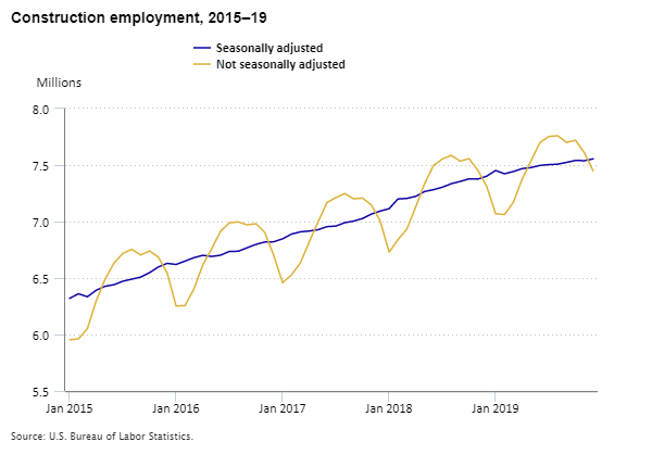
Editor’s note: Data for this chart are available in the table below.

BLS seasonally adjusts data in several of its monthly and quarterly news releases.

• National Employment and Unemployment (monthly)
• State Employment and Unemployment (monthly)
• Metro Employment and Unemployment (monthly)
• Job Openings and Labor Turnover (monthly)
• Consumer Price Index (monthly)
• Producer Price Indexes (monthly)
• Employment Cost Index (quarterly)
• Labor Productivity and Costs (quarterly)
• Business Employment Dynamics (quarterly)

Two Approaches to Seasonal Adjustment

BLS uses one of two approaches to seasonally adjust data in these releases—projected factors or concurrent seasonal adjustment. When we project seasonal adjustment factors, we only use historical data in the models. That means we calculate factors in advance, so they are not influenced by the most recent trends. Concurrent seasonal adjustment uses all the data available, including the most recent month or quarter. As a result, the factors are influenced by recent changes.

Regardless of whether the factors are projected or concurrent, the seasonal adjustment models can be additive or multiplicative. We’ll explain more about that below. The COVID-19 pandemic affected the seasonal adjustment process in different ways depending on how the seasonal factors are calculated.

Approach #1

The Consumer Price Index, Producer Price Indexes, and Employment Cost Index use the projected-factor approach and calculate seasonal factors once a year. BLS staff estimated the 2020 seasonal factors at the beginning of 2020 and have used them throughout the year. When new factors for 2021 and revised historical factors are calculated, BLS will examine the effects of the pandemic on the seasonal adjustment models.

Approach #2

We use a concurrent process to calculate the seasonal factors each month for nonfarm employment estimates for the nation, states, and metro areas, unemployment and labor force estimates for the nation, states, and metro areas, and job openings and labor turnover estimates. Each quarter, BLS also uses a similar concurrent process to calculate seasonal factors for productivity measures and business employment dynamics. This helps create the best seasonal factors when seasonality may shift over time. For example, think of schools letting out for summer a little earlier than they usually do each year, or the changing nature of delivery services because of online shopping. Using the most recent data to calculate seasonal factors helps pick up these changes to seasonality faster than the forecasted method. The risk of using the concurrent process is that it may attribute some of the movement in the estimates to a changing seasonal pattern when it really resulted from a nonseasonal event. BLS also annually examines and revises the historical seasonal factors even if the factors were originally calculated using concurrent adjustment. As the saying goes, hindsight is 20/20.

Before the COVID-19 pandemic, the concurrent seasonal adjustment models required limited real-time intervention. Examples of potential reasons for intervention include major events like hurricanes. The COVID-19 pandemic is unusual in its severity and duration, so significant intervention was needed.

BLS intervened in several ways to create the highest quality, real-time seasonal factors. The tool we use most often is called outlier detection. We consider outliers not to represent a normal or typical seasonal movement. When we label an observation as an outlier, we don’t use it to inform the seasonal adjustment model. Since economic activity is still being heavily influenced by COVID-19 and efforts to contain it, BLS has detected more outliers. When this happens, concurrent models behave more like projected-factor models because the most recent data are not used to create seasonal factors.

The Local Area Unemployment Statistics program uses another type of intervention, a technique call a level shift. It is used when there is a sudden change in the level of a data series. In this case, level shifts were used over a series of months.

Additive versus Multiplicative Models

As noted earlier, all BLS programs review their seasonal adjustment models each year. One of the steps during this process is to select a model—either additive or multiplicative. We use an additive model when seasonal movements are stable over time regardless of the level of the series. A multiplicative model is better to use when seasonal movements become larger as the series itself increases—that is, the seasonality is proportional to the level of the series. That means a sudden large change in the level of a series, such as the large increase in the number of unemployed people in April 2020, will be accompanied by a proportionally large seasonal effect. BLS did not want this to occur. When there are large shifts in a measure, multiplicative seasonal adjustment factors can result in adjusting too much or too little. In these cases, additive seasonal adjustment factors usually reflect seasonal movements more accurately and have smaller revisions.

Because of the unusual data patterns beginning in March 2020, both the Current Population Survey, which we use to measure unemployment and the labor force, and the Job Openings and Labor Turnover Survey switched from multiplicative to additive seasonal models for most series and did not wait until the typical yearend model review.

BLS does not produce the weekly data on unemployment insurance. We do, however, compute the seasonal adjustment factors used by the Department of Labor’s Employment and Training Administration for their Unemployment Insurance Weekly Claims data. As we recommended, the Employment and Training Administration recently switched from using multiplicative to additive seasonal adjustments.

Our quarterly Labor Productivity and Costs news release uses input data from the Bureau of Economic Analysis, the U.S. Census Bureau, and several BLS programs. Most of the input data are already seasonally adjusted by the source agencies or programs. The productivity program only seasonally adjusts monthly Current Population Survey data on employment and hours worked for about ten percent of workers, mostly the self-employed, who are not included in the monthly data from the Current Employment Statistics survey on nonfarm employment and hours. The productivity program detected outliers in some of the data beginning at the start of the COVID-19 pandemic in March 2020 and accounted for them in the estimates.

Science and Art

Seasonal adjustment of economic data is a scientific process that involves complex math. But seasonal adjustment also involves some art in addition to science. The art comes in when we use our judgment about outliers in the data or when we decide whether an additive or multiplicative model more closely reflects seasonal variation in economic measures. The art also comes in when we recognize how complicated the world is. During 2020 we have experienced not just a global pandemic but also massive wildfires in several western states, a historic number of hurricanes that made landfall, and other notable events that affect economic activity. Did our seasonal adjustment models properly account for all of these events? I can say we have tried our best with the information we have available. As we gather more data for 2020 and future years, we will continue to examine how we can improve our models to help us distinguish longer-term trends from the seasonal variation in economic activity.

Acknowledgment: Many BLS staff members helped make the technical details in this blog easier to understand, and they all have my gratitude. Three who were especially helpful were Richard Tiller, Thomas Evans, and Brian Monsell.