
An official website of the United States government
An official website of the United States government
The .gov means it's official.
Federal government websites often end in .gov or .mil. Before sharing sensitive information,
make sure you're on a federal government site.
The site is secure.
The
https:// ensures that you are connecting to the official website and that any
information you provide is encrypted and transmitted securely.
The distribution of economic well-being has been the focus of researchers and followers of economic indicators for many years, with economic well-being most often defined in terms of income, expenditures or consumption, and wealth. This note outlines methods developed by the U.S. Bureau of Labor Statistics (BLS) to distribute personal consumption expenditures (PCE) as a counterpart to the BEA distribution of Personal Income (PI) product by Fixler et al. (2017, 2020) and Gindelsky (2023). This document also includes some analysis that supplements the tables posted to the BLS webpage. For an earlier version of the analysis with more details and background information, see Garner, et. al. (2022).2 All results in this report are based on PCE data released on September 26, 2024.
The overall strategy is to use Consumer Expenditure Surveys (CE) microdata to describe the distribution of PCE across households in the U.S., or in the case of the CE, consumer units. Doing this requires not only matching comparable categories across statistical series, but also adjusting less-comparable CE categories of expenditures so that they better match PCE definitions, deleting expenditure items that are out-of-scope for PCE, and imputing expenditures for items that are out-of-scope for CE. The base of the analysis is the quarterly CE Interview Survey, for which we source about 94% of CE spending which is eligible for PCE (based on 2019 data). For some categories, the CE Diary is either the sole (e.g., postage stamps, non-prescription drugs) or more reliable in our judgement (e.g., clothing and footwear) source of expenditure reports. A statistical matching procedure imputes these Diary expenditures to the CE Interview sample. Once a set of comparable and augmented CE data are assembled, PCE spending shares by deciles of equivalized total expenditures are computed as well as distributional statistics (such as the ratio of the 90th to the 10th percentile and Gini coefficient) for total expenditures and total equivalized expenditures. Equivalized expenditures are calculated by dividing consumer unit total expenditures by the square root of the number of people within the consumer unit.
The process of combining CE and PCE data to create distributions of PCE is summarized as follows.
The following section describes many of the inherent issues and challenges in further detail.
A first step in producing the distributional statistics is to adjust data. This is necessary as there are differences in the CE and PCE that are based on the purpose of each and thereby the populations covered.3 The CE is designed to collect out-of-pocket spending on goods and services (e.g., food, health insurance) or the acquisition costs (e.g., the purchase of vehicles) by consumer units living in the U. S. in noninstitutional setting (with the exception of students living in college or university housing which are included in the CE sample). In contrast, the PCE reflects purchases of goods and services made by and on behalf of households (including by the federal government) and by non-profit institutions serving households (NPISHs). For this study we distribute PCE (for 150 categories from NIPA Table 2.4.5U) across consumer units using data from the CE. We only explicitly distribute the components of the PCE that exclude expenditures by NPISHs to more closely match the types of expenditures and population covered by the CE. 4 However, to match the PCE tables, we publish topline PCE estimates (including means, medians, and shares) which have NPISH spending included. To get these aggregates, the NPISH spending is assumed to be distributed the same as the household consumption expenditure portion of PCE, so as to not affect the overall PCE distribution. While this assumption is strong, the CE data do not include data on receipts of such benefits.
The PCE covers a broader set of goods and services than does the CE; the PCE focuses on expenditures for what is produced within a year in line with the National Income and Product Accounts (NIPA). The CE reflects consumer unit purchases from private and public establishments, and in addition, purchases from other consumer units through household-to-household transactions (e.g., for used cars). In contrast, the PCE reflects purchases from private businesses, costs incurred by NPISHs in providing goods and services on behalf of households, and purchases made by third-party payers on behalf of households. Third-party payer expenditures include those for employer-paid health insurance, medical care financed through government programs, and financial services (such as banking services) that benefit households but for which they do not pay directly. 5 However, in contrast to the CE, household-to-household transactions are excluded from the PCE.
The CE comprises two surveys, an Interview and Diary, each with its own sample of consumer units. The Interview Survey has a three-month recall period and is designed to cover larger expenditure purchases (e.g., major appliances) and recurring items (e.g., rent, utilities). Consumer units are interviewed once every three months for up to four consecutive quarters on a rolling basis. In contrast, the Diary is designed to cover smaller expenditure, such as prescription drugs, and frequently purchased items, such as detailed food. For these goods and services, data are collected over two consecutive weeks using one-week diaries.
The Interview and Diary overlap in coverage for some categories, though sometimes at differing levels of aggregation or frequency. As consumer unit-level expenditures are the building blocks of this analysis, we generally choose the Interview as the source when both surveys have coverage. We estimate total expenditures from the CE that are as close to PCE definitions as possible, and out of these we find about 94% can be represented by the Interview in 2019, and expect for similar results for other years. This results in a remainder of about 6% for which the Diary is the only source or the most-reliable source by our judgment.6
For a given calendar year, we start with the set of quarterly CE interviews that were collected from the first quarter through the first quarter of the next calendar year. The staggered timing of CE interviews, combined with missing data, means a relatively small sample give annual expenditures for an exact calendar year. To form a larger sample, we include all consumer units whose expenditure reference periods started as early as November of the prior year or ended as late as February of the following year, provided they completed at least two quarterly interviews. This yields a sample of 8,238 consumer units in 2017, 7,717 in 2018, 7,171 in 2019, 6,734 in 2020, 6,726 in 2021, 6,310 in 2022, and 6,250 in 2023. For consumer units who completed fewer than four quarters, we scale their expenditures up to represent one year of expenditures
We also recalibrate the sampling weights to match calendar year counts and average demographic characteristics from the Current Population Survey (CPS). The BLS usually calibrates CE data to 35 controls or known totals of people and households in the civilian non-institutional U.S. population; the known totals are from the CPS. The controls are counts based on certain geographic and demographic variables, with some being people counts and others being household counts. These include, for 2020 onward, 14 age/race groups, 9 Census divisions, 9 urban Census divisions, the total number of Hispanics, the total number of owners, and the total number of households. The latter two controls are household counts; the BLS converts these household counts to CE consumer unit counts by factoring in a relatively small adjustment.
This project requires modifications to the normal CE calibration process. The CE normally treats each consumer unit independently in a quarterly weighting process, with a consumer unit defined as having participated in any one of its four quarterly interviews. However, we use interviews from an expanded period as noted earlier (part of the first quarter of the calendar year through part of the first quarter of the subsequent calendar year), with a consumer unit defined as having participated during that period in either 2 of its 4 quarterly interviews, 3 of its 4 quarterly interviews, or all 4 of its quarterly interviews. This special way of defining a consumer unit means that we generate only one set of calibrated weights for each consumer unit, no matter if it completed two, three, or four quarterly interviews. Our calibrations averaged the 35 controls from the CPS data over the period that the data were collected, rather than over three months. Lastly, we adjusted the weights for the set of quarterly CE interviews used in this project since the data are a subsample from five quarters of CE’s collected data. This adjustment ensures the sum of the weights match the number of consumer units in the population in the intended calendar year.
We start with the monthly expenditure (MTAB) files from the CE and map spending to PCE categories, as described in the following subsection. After mapping CE expenditures to the PCE categories and imputing some missing categories, we scale expenditures so that population totals for 150 detailed categories match the PCE estimates from NIPA Table 2.4.5U.
As stated, we match the CE microdata to the definitions of the PCE categories to the greatest extent possible. We start from a mapping of CE spending categories, called Universal Classification Codes (UCC) to PCE categories or product types.7 BLS maintains a similar mapping for comparison purposes (Bureau of Labor Statistics, 2023). We map, allocate, or impute spending for 150 detailed PCE categories. We are not always able to match CE and PCE to the most disaggregated PCE data, which consists of 244 separate categories in NIPA. Some detailed categories have no counterpart in the CE (e.g., 22 categories for NPISH), and some are either more disaggregated in PCE (e.g., foreign vs domestic autos) or have spotty coverage in the CE due to sample size (e.g., pleasure aircraft).
Some additional details on this mapping and imputations are introduced in the subsections below. The procedure used to distribute financial services furnished without payment, securities commissions, portfolio management and investment advice services, trust, fiduciary, and custody activities, income loss insurance, and worker's compensation insurance is similar to McCully (2014) in that some of the PCE amount are distributed using a noncomparable CE series (e.g., pension contribution) as an indicator. They differ from McCully (2014) in that our methods use only published PCE amounts and only CE microdata (McCully also used wage data from the Current Population Survey Annual Social and Economic Supplement).
The CE published estimates for new and used automobiles subtract trade-in allowances from sales prices. To better reflect PCE aggregates, we add back in the trade-in values for new vehicle purchases. We then subtract these trade-in allowances from used vehicle spending under the assumption that vehicles traded in are eventually resold to the household sector, and as such, more closely align with the definition of new and used automobiles in the PCE. For this analysis, CE used vehicle expenditures do not include those that reflect household to household transactions for consistency with the PCE. Section 3.C discusses the impact of alternative treatments of used vehicles on the analysis.
PCE includes imputed financial services—such as free checking accounts and online record-keeping—which benefit consumer units, but CE does not capture because they are not purchased explicitly. We distribute the PCE amount for these services assuming they are proportional to the value of balances held at commercial banks and other depository institutions, as well as pension fund contributions. Similarly, we distribute the PCE for commissions on securities purchases and sales, portfolio and investment advice services, and trust, fiduciary, and custody activities using CE data for the market value of securities held. The CE only collects this financial information in the fourth interview, which is missing for some consumer units due to attrition. To impute values for these missing units, we use a statistical matching procedure based on other observations in the same income quartile.
Through 2022, the Interview survey data files include only global aggregates for “at home food and non-alcoholic beverages” and “at home beer, wine, other alcohol.” For 2023, the “at home food and non-alcoholic beverages” series was replaced a global question on expenditures from grocery stores, of which we map a fixed proportion (80%) to PCE (following the method used for the published CE tables). We use matched Diary observations (see Section 2.D) to allocate these global expenditures across the 21 detailed food and beverage categories from NIPA Table 2.4.5U. We also impute the PCE category “food produced and consumed on farms” by distributing the PCE total across consumer units living on farms, proportionally to their family size. Starting in 2023, a combined food and alcoholic beverages from restaurants series in the CE Interview was used to distribute the PCE for restaurant meals (“other purchased meals”), while the Diary was used for the PCE for alcohol in purchased meals.
Table 2.1 summarizes the imputation procedures and data sources for health care.8 The comparison of CE and PCE health care expenditures is complicated by two issues. First, the scopes of the CE and PCE differ. Before the CE can be mapped to the PCE, expenditures that are out of scope in the CE must be imputed to consumer units. Second, the health care expenditure categories in the PCE are defined differently than in the CE, and adjustments must be made to the CE expenditures as some items that are classified as health expenditures in CE get mapped to non-health categories in the PCE.
| Type | For Whom | Value of Imputation | Source of data |
|---|---|---|---|
|
Public |
|||
|
Medicare |
Assigned to consumer unit (CU) members enrolled in Medicare | National average benefits scaled by state level spending differences | CMS 2020 Medicare Trustees Report (https://www.cms.gov/files/document/2023-medicare-trustees-report.pdf) |
|
Medicaid |
Assigned based on the number of CU members identified as participating | National average expenditures per enrollee scaled by state level spending differences | CMS National Health Expenditures (NHE) |
|
CHIP |
Assigned based on the number of CU members identified as participating | National average expenditures per enrollee | CMS National Health Expenditures (NHE) |
|
Other public (VA, Tricare, and other military, and IHS) |
Assigned based on the number of CU members identified as participating | National average expenditures on private care | Agency Budgets |
|
Private |
|||
|
Employer provided |
Assigned to each CU reporting employer coverage based on the number of individuals covered: self only (number covered = 1), self plus one (number covered = 2), family (number covered >2) | State average premium paid by employer for health insurance by policy type (self only, self plus one, family) | MEPS-IC (https://datatools.ahrq.gov/meps-ic) |
|
Individual |
Assigned to each CU reporting individual coverage and receiving a subsidy (subsidy receipt is imputed for 2014) | State average premium tax credit among those who receive a credit | CMS (https://www.cms.gov/files/document/ehttps://www.cms.gov/files/document/early-2023-and-full-year-2022-effectuated-enrollment-report.pdf) |
Notes: The most up-to-date estimates available are used. For private insurance, the imputed amounts are added to out-of-pocket premiums reported in the CE. For other public plans, only care provided in non-government facilities is in scope for the PCE. The VA and IHS budgets include these amounts as a separate line item. The Department of Defense submits a separate budget for care purchased from private providers for Tricare. The state average premium paid by employers is an enrollment-weighted average of state-level average contributions for private sector employees with Census division average contributions for state and local government employees, assuming state-level enrollment for state and local government employees is proportional to state-level employment. Prior to 2017, CE did not ask separate questions about CHIP, VA, or other military health coverage.
The scope of the health care categories differs greatly between the CE and PCE. The CE only includes out-of-pocket spending for health insurance and health care goods and services. In contrast, the PCE in addition includes expenditures by employers and the government on behalf of consumers which we impute using external sources.9 For employer contributions to health insurance premiums, we use Medical Expenditure Panel Survey – Insurance Component (MEPS-IC) data to compute average employer contributions by plan type (self, plus one, and family) and State. For plans purchased in the individual market, we add the average tax credit by state to the out-of-pocket premiums for individuals who report receiving a subsidy10. No adjustments are made for those who purchase unsubsidized plans in the individual market. For Medicaid and Child Health Insurance Program (CHIP), we use the average expenditures per enrollee from the National Health Expenditure (NHE) Table 21. For Medicaid, we apply state-level factors based on data from Center for Medicare and Medicaid Services (CMS). For Medicare, we compute the average expenditure per enrollee for traditional Medicare (parts A and/or B), Medicare Advantage (part C), and prescription drug coverage (part D) using Boards of Trustees (2023). We use state-level Medicare spending data to scale these values by state and add these amounts to the out-of-pocket premiums included in the CE data for part C which capture the out-of-pocket premium in excess of the part B premium. Other government programs (Indian Health Service, CHAMP-VA, and Tricare) provide much of the care at government owned and operated facilities, which are out of scope for the PCE. Care provided in non-government owned facilities through these programs are in scope, so we use the average expenditure for private providers per enrollee for these programs.11 The per enrollee amounts are multiplied by the number of covered members in the consumer unit.
Once the total premium expenditures are imputed for the CE, some adjustment must be made to CE health expenditures to match the category definitions in the PCE. With the imputations for employer and government contributions to health insurance, CE health insurance expenditures include the total premiums and are categorized as health expenditures along with out-of-pocket spending on medical goods and services. Health insurance in the PCE measures net premiums (premiums minus benefits) and is categorized as a financial service. As defined for the PCE, spending on medical goods and services includes the total amount paid to the providers (out-of-pocket payments plus any insurance reimbursement), while CE only includes out-of-pocket spending. The medical care category in the CE includes medical goods and medical services (including insurance). In contrast, in the PCE (Table 2.4.5U), some medical goods (e.g., therapeutic appliances and equipment) are categorized as durables, others as non-durables (e.g., pharmaceutical products), and other as health care services. The health care product category in the PCE as presented in Table 2.3.5 includes non-insurance medical services only.
Before the CE can be mapped to PCE, health insurance premiums that go towards benefits need to be reassigned to medical goods and medical services. The remaining premium amount reflects the net premiums and can be mapped to the health insurance category in the PCE. Thus, total health insurance premiums in the CE are allocated across up to twelve different PCE categories: therapeutic medical equipment, prescription drugs, other medical products, physician services, dental services, home health care, medical laboratories, specialty outpatient care, all other professional medical services, hospitals, nursing homes, and net health insurance. Data from the National Health Expenditure Accounts (NHE) as well as the BES's PCE bridge tables12 are used to reassign total premiums into these categories based on the type of insurance.
The CE only collects information on out-of-pocket tuition payments by consumer units, while PCE is based on the receipts and outlays of colleges and universities and implicitly, therefore, includes scholarships, grants, and payments made on behalf of students from all sources including government, private, and non-profit. We distribute the college tuition PCE, minus the CE amount, proportionally to the number of college students in the household.
The PCE for net household insurance includes coverage for renters, condominium/cooperative owners, and a portion of independent owners’ premiums reflecting coverage for the loss of contents (but not for the loss of the structure). For CE homeowner’s insurance premiums, we use an adjustment factor to reflect this scope difference. Unlike for motor vehicle and medical insurance, we do not allocate premiums between net insurance and goods and services spending, due to data limitations. The net insurance PCE total is therefore distributed based on household’s total out-of-pocket premiums.
Housing services PCE for owner-occupiers are measured using the rental equivalence concept, which is measured in the CE. When data are available (2009 and later), we make adjustments if consumer units have partial ownership, rent out secondary residences part of the year, or if they use part of the home for business. The BLS also adjusts for partial ownership and vacation rentals when weighting the Consumer Price Index. PCE also separates tenant rents and implicit rents between nonfarm and farm properties. For farms, tenant rents and implicit rents are combined into one category. For consumer units living on farms, we map their primary residence to this category. Finally, some renters in the CE have some utilities included in their rent payment. We allocate a portion of their rent payment to the various utilities categories using a factor based on the average rents of those which include utilities and those which do not.
As with other insurance products, the PCE category for motor vehicle insurance reflects only the net premium (total premium minus normal losses) while various PCE categories include payments by insurance companies on behalf of households. Therefore, like for health insurance, we allocate insurance premiums between net insurance and different goods and service categories. We allocate across four categories: motor vehicle accessories and parts, motor vehicle repair services, hospital services, and net motor vehicle insurance. We use data from the National Association of Insurance Commissioners (NAIC, 2024) averaged for 1999-2019, as well as relative PCE totals to make the allocations. Averaged data (excluding 2020 as an outlier) was chosen to better reflect the PCE net premium concept of “normal losses.”
As previously mentioned, PCE includes the final consumption expenditures of non-profit institutions serving households. After all other imputations and adjustments, we distribute total NPISH spending neutrally, that is, proportionally to non-NPISH PCE, so that it has no impact on the distribution.
PCE includes subtractions (NIPA Table 2.4.5U lines 149 and 338) for expenditures of nonresidents, as these are not separable from other category totals (e.g., food services and accommodation). As nonresidents are not part of the CE sample, we treat these lines similarly to NPISH and distribute the subtractions neutrally. For spending abroad by U.S. residents, we distribute the PCE total using spending on passenger fares for foreign travel as an indicator.
PCE categories for social assistance, social advocacy and civic and social organizations, religious organizations’ services to households, and foundation and grantmaking and giving services to households do not have close counterparts in the CE (similarly named cash contribution series in the in the CE far exceed PCE aggregates and largely reflect transfers rather than consumption expenditures). We allocate these PCE totals neutrally, similar to NPISH spending.
We distribute PCE amounts proportionally to using wages and salaries from the CE. These are collected in the first and fourth interviews, and BLS carries over values from the first interview to the second and third interview when producing the datafiles.
For this study, we were able to adjust CE to account for some differences, but not all. We redefined CE expenditure categories to follow those of the PCE as much as possible. For example, for comparability to the PCE, rental equivalence as collected in the CE is used as in the published comparisons between CE and PCE.13 This contrasts the CE published tables of means, which use some out-of-pocket shelter expenditures.14 In addition, household-to-household transactions (e.g., for vehicles) are dropped from the CE expenditures. Our efforts to adjust CE data for education spending from NPISHs or the government are limited to the procedure described in Section 2.B.4.
We were only able to partially adjust for the differences due to CE and PCE population coverage. As mentioned, the BEA produces aggregates for households and NPISHs, and we only explicitly distribute the household consumption portion. The NPISH portions are defined as gross output of NPISHs minus the receipt of sales of goods and services by NPISHs, and we have no way to link these with potential beneficiaries. With the exceptions noted below, both the CE and PCE populations consist of households that reside (at least one year) in the U.S. regardless of country of origin. The PCE population also, government employees and private employees living abroad; these households are not included in the CE population. However, included in the CE population but not the PCE are foreign students if they have a U.S. address or live in U.S. college or university housing. We do not make any adjustments to PCE totals for residents traveling abroad or domestic spending by nonresident households.
We implement a statistical matching procedure based on Hobijn et al. (2009) to impute the remaining 6% of PCE-eligible spending not sourced from the Interview Survey. Similar donors from the Diary sample provide the missing data for each Interview consumer unit, where similarity is determined by a model of monthly expenditure as a function of demographic characteristics.15 The model provides a convenient method of weighting a relatively large number of characteristics by doing so according to which linear combination most strongly predicts expenditures. We then use the predicted values to form measures of distance between Interview consumer units and prospective Diary donors. The only characteristic guaranteed to match between donor and recipient is quintile of the annual before-tax income distribution.16 The matching procedure is many-to-one, as we draw four donor Diaries for each Interview in each month with replacement.17
First, we stratify both Interview and Diary consumer unit samples by quintiles of annual before-tax income.18 The rankings of income are done separately for each survey. CE started imputing missing income sources in 2004. For prior years, we use a similar multiple imputation procedure based on Fisher, et al. (2014)19. For each expenditure reference month 𝑡 and quintile 𝑞, we use the Interview sample to estimate the regression
where yht is logged expenditure of consumer unit h, uht is an error term, and xht include Census region, urban/rural, age, race, sex, and education of the reference person, consumer unit size, and the prior year’s annual before-tax income.20 For the model, the measure of expenditure we use is the total monthly expenditure of the Interview household after mapping to PCE product definitions, but before imputations for employer or publicly provided health care.21 We use the least squares estimator weighted by the CE sampling weight, finlwt21.
Let

be the slope estimate for quintile 𝑞 in month 𝑡. As household characteristics are available and comparably defined in both surveys, we calculate predicted values
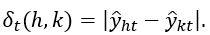
for each Diary and Interview observation. For a given Interview observation ℎ and Diary observation 𝑘, the distance metric is defined as
Within each month and income quintile, we calculate δt for all {ℎ,𝑘} pairs. Then for each Interview observation ℎ, we randomly select (with replacement) four 𝑘 from the twenty smallest δt out of all the Diary observations from the same month and income quintile. The random component is intended to ensure a more even distribution of matches across Diary observations. The detailed set of expenditures (after adjustments to match PCE definitions) of the donor Diary is then assigned to the recipient Interview. As one donor Diary is intended to represent one quarter of one month of expenditure, but Diaries correspond to a one-week reference period, the donor Diary expenditures are scaled by 13/12. This process is repeated for each Interview observation, for each month it is in the sample.
Even after imputations to capture spending which is out-of-scope to the CE, the sum of CE spending (including the imputations) does not equal total PCE. In addition, it is possible that the remaining "missing" PCE is not distributed proportionally to the observes expenditures, so that the data might understate inequality in consumption expenditures. To mitigate this, we follow the suggestion in Zwijnenburg, et al. (2022) by making draws from a type-I Pareto distribution. The distribution is applied to the top 5% of consumer units ranked by total spending after adjustments and imputations, but before scaling to match NIPA totals. We used a shape parameter of 2 based on Zwijnenburg, et al. (2022) and our judgement. The Pareto draws are used to scale-up spending on the top 5%, excluding imputed categories which already match NIPA totals by construction (e.g., financial services furnished without payment).
After allocating CE to PCE categories and imputing missing items, we then sum expenditures for each consumer unit to the PCE major product level. CE aggregates differ from PCE aggregates for most categories. Table 3.1 describes the extent to which CE and PCE differ after adjustments, allocations and imputations. Before adjusting for these discrepancies, we impose a lower bound of zero on expenditures at the major product-level which affects a small number of observations.22
To allocate PCE expenditures across the distribution of equivalized total expenditures, as defined above, a next step is needed to close the remaining gap between CE and PCE. CE expenditures are scaled up to consumer unit-level PCE estimates so that totals match BEA’s published estimates for 150 detailed categories from NIPA Table 2.4.5U.23 This scaling is referred to as a proportional adjustment and reflects the allocation of the gap between CE and PCE totals in proportion to the underlying micro data.24 For example, if aggregate PCE for physician's services equals $551 billion and consumer unit X had 0.000005% of total CE physician's services expenditures (after imputations for health insurance and allocations to PCE categories), consumer unit X is assigned 0.000005%*$551 billion as its total physician's services expenditure. The scaling implicitly distributes the “missing” product-level expenditures identically to those already captured by the CE. Ideally, we would aim to use supplementary data to make imputations to narrow the gaps as much as possible before scaling. Our initial efforts in this area focused on healthcare, where government and employer provided benefits have a much more equal distribution than out-of-pocket spending captured in the CE. See Garner, et. al. (2022) for more details. Since then, we have added further imputation (see subsection 2.B), including for financial services furnished without payment, which have a much less equal distribution than out-of-pocket spending.
To create the deciles across which to distribute the PCE expenditures, we rank consumer units based on their total expenditures equivalized by the square root of family size as the equivalence scale. In creating the ranking (as a precursor to creating quantile groupings), consumer units are weighted by their CE sampling weight (finlwt21).25 Total expenditures are defined as the sum of aggregate expenditures based on PCE major product type after all the processing described in Section 2.B to match PCE definitions and impute spending not covered by CE (e.g., health care), and after scaling up expenditures to PCE totals as described in Section 2.F.
Starting with the December 2024 release, we estimate PCE price indexes and market-based PCE price indexes by decile of equivalized PCE (as defined in Section 2.G.). Market-based PCE excludes categories such as imputed financial services, but does include imputed rent from owner-occupied housing. To construct group-specific PCE price indexes, we combine the detailed PCE price subindexes from NIPA Table 2.4.4U with decile-specific expenditure shares. Matching BEA’s method, we use the chained Fisher formula, which combines current and prior-year expenditure shares. As discussed in Section 2.B, we distribute 150 detailed components, but some of these cover more than one of the 244 most detailed categories in NIPA Table 2.4.5U. In these cases, to take new automobiles as an example, our price indexes reflect differences across groups in spending shares on new automobiles out of all goods and services, but not spending share differences on foreign vs. domestic automobiles (which are not so delineated in the CE). Finally, note that the Fisher formula is not additive, so the sum of chained dollar PCE estimates across all subgroups will not exactly equal total chained dollar PCE.
Figure 3.1 below summarizes the relative contribution of the raw CE data and various imputation procedures within each decile of equivalized PCE. Raw CE data make up 46-55% of PCE within PCE-defined deciles, with imputations accounting for 18-26%. The Pareto adjustment comprises about 9% of PCE for the top decile, while proportional allocation accounts for between 21 and 25%.
Figures 3.2 and 3.3 show the amount of imputations for 2019, by decile of total equivalized PCE. Health care is the largest source of imputation for each decile and is flat starting with the third decile. Imputed financial services are small at the lower end of the distribution, but large for the top decile.
Table 3.1 below shows the ratios of CE to PCE aggregates before the scaling to match PCE product type totals. See Garner, et. al. (2022) for more details on the impact of the allocation and imputation of health care spending on the PCE coverage rates. For example, for all categories in 2019, the CE/PCE ratio is 0.76. For Durable Goods, it is 0.62, for Non-Durable Goods, it is 0.67, and for Services it is 0.82. The ratio for Housing and Utilities is 1.09 in 2019. That this is greater than unity is largely due to owner equivalent rent. In the CE-PCE comparison conducted by the CE Program as part of data comparisons, the same owner equivalent rent is used but the CE Program published ratio is 1.17 due to no adjustment by ownership or use. The BEA bases their measure on an imputation model based on actual rents plus an owner’s premium (Rassier, et al. 2021). See also Garner and Short (2009) for more on this topic.
| Category | 2019 | 2020 | 2021 | 2022 | 2023 |
|---|---|---|---|---|---|
|
PCE less final consumption expenditures of nonprofit institutions serving households |
0.76 | 0.78 | 0.74 | 0.74 | 0.74 |
|
Durable goods |
0.62 | 0.63 | 0.6 | 0.55 | 0.54 |
|
Motor vehicles and parts |
1.01 | 1.03 | 0.84 | 0.82 | 0.91 |
|
Furnishings and durable household equipment |
0.55 | 0.53 | 0.52 | 0.55 | 0.44 |
|
Recreational goods and vehicles |
0.25 | 0.33 | 0.46 | 0.28 | 0.22 |
|
Other durable goods |
0.45 | 0.45 | 0.44 | 0.46 | 0.4 |
|
Nondurable goods |
0.67 | 0.64 | 0.62 | 0.65 | 0.63 |
|
Food and beverages purchased for off-premises consumption |
0.75 | 0.74 | 0.73 | 0.77 | 0.72 |
|
Clothing and footwear |
0.5 | 0.44 | 0.38 | 0.4 | 0.43 |
|
Gasoline and other energy goods |
0.85 | 0.87 | 0.81 | 0.87 | 0.82 |
|
Other nondurable goods |
0.6 | 0.56 | 0.53 | 0.54 | 0.55 |
|
Household consumption expenditures (for services) |
0.82 | 0.85 | 0.81 | 0.81 | 0.81 |
|
Housing and utilities |
1.09 | 1.09 | 1.11 | 1.12 | 1.1 |
|
Health care |
0.81 | 0.86 | 0.78 | 0.78 | 0.79 |
|
Transportation services |
0.59 | 0.64 | 0.58 | 0.56 | 0.53 |
|
Recreation services |
0.42 | 0.44 | 0.43 | 0.41 | 0.4 |
|
Food services and accommodations |
0.54 | 0.46 | 0.53 | 0.58 | 0.61 |
|
Financial services and insurance |
0.92 | 0.96 | 0.89 | 0.91 | 0.93 |
|
Other services |
0.65 | 0.65 | 0.59 | 0.61 | 0.62 |
Note: Data represent CE divided by PCE as published in BEA NIPA Table 2.3.5 (September 26, 2024 release).
Researchers have used various weighting options for the production of distributional statistics (e.g., percentile ratios like the 90/10 and aggregate indexes like the Gini). For example, de Queljoe et al. (forthcoming 2025) and Gindelsky (2020) weighted equivalized expenditures using household or consumer unit weights (finlwt21 for the CE) following the EG DNA guidelines.26 The reasoning for selecting this option is that households, not people, are the focus of income and consumption expenditure national accounts. In contrast, the OCED ICW expert group (OECD 2013) recommended that the use of person-weighting when producing distributional statistics based on an economic unit (e.g., household, consumer unit, family) or any other statistical unit that combines individuals. The assumption with this weighting option is that equivalized household income or expenditures are available to each person in the household. In the case of the CE, the person-weight would be defined as finlwt21 times consumer unit size. Another option is to weight by the number of “consumption units”; this is the number of equivalized adults times the household or consumer unit weight. The number of equivalent units is a function of the equivalence scale chosen. For example, with the equivalence scale being the square root of consumer unit, a 2-adult household is represented by 1.41 equivalent units (times the consumer unit population weight). When conducting distributional statistics, this latter weighting option ensures that the sum of equivalized expenditures within a decile, for example, equals the total expenditure for the decile.
In our estimates, we use finlwt21 (the CE sampling weight) for computing statistics concerning equivalized PCE and for the creation of decile and other quantile groups (e.g., the 10%-20% group).27 We study alternative weights—finlwt21 times family size and finlwt21 times the square root of family size. We find a minor quantitative impact, which is shown in Table 3.2. The effects of including family size in the weight are a slight decrease in the mean and median and a slight decrease in the share accounted for by the top decile and percentiles. Summary measures like the Gini index are constant (to two decimal places), while the 90/10 ratio is slightly lower (3.49 vs. 3.54). Garner, et. al. (2022), in Appendix A, show the impact of the weight change on the deciles of total equivalized expenditure.
| Statistic / Weight | finlwt21 | finlwt21*sqrt(fam_size) | finlwt21*fam_size |
|---|---|---|---|
|
Equivalized total mean |
$73,272 | $72,586 | $71,324 |
|
Equivalized total median |
$60,478 | $59,774 | $58,316 |
|
Equivalized total: 0-20% share |
8.80% | 8.80% | 8.80% |
|
Equivalized total: 20-40% share |
12.90% | 12.90% | 12.90% |
|
Equivalized total: 40-60% share |
16.50% | 16.40% | 16.40% |
|
Equivalized total: 60-80% share |
21.30% | 21.20% | 21.20% |
|
Equivalized total: 80-100% share |
40.50% | 40.70% | 40.80% |
|
Equivalized total: 80-99% share |
33.70% | 33.80% | 33.70% |
|
Equivalized total: Top 1% share |
6.80% | 6.90% | 7.00% |
|
Equivalized total: Top 5% share |
17.50% | 17.80% | 17.90% |
|
Equivalized total: 90/10 |
3.54 | 3.53 | 3.49 |
|
Equivalized total: Gini index |
0.31 | 0.31 | 0.32 |
|
Equivalized total: Theil index |
0.2 | 0.2 | 0.21 |
|
Equivalized total: Log-Deviance |
0.16 | 0.17 | 0.17 |
|
Equivalized total: CV |
0.35 | 0.36 | 0.37 |
Notes: Columns track changes in distributional statistics when different weights are used to both to create quantile groups and weight the statistics. Finlwt21 is the sampling weight used by CE, adjusted for our sample of interviews. “fam_size” refers to the number of members of the consumer unit.
Table 3.3 below presents results under alternative treatments of used motor vehicles compared against the baseline results in column (1). The baseline processing rules of excluding purchases which originated from another household and subtracting sales made by the consumer unit most closely match PCE definitions. Indeed, these rules produce CE aggregates which come closest to PCE totals (ratios close to unity). Subtracting sales has relatively minor effect on the distributional results, while excluding household-to-household purchases shifts the distribution of expenditures slightly toward the lower quantiles of equivalized PCE once recalculated.
| (1)* | (2) | (3) | (4) | |
|---|---|---|---|---|
|
Processing Rules |
||||
|
Exclude used purchases from households |
Yes | Yes | No | No |
|
Subtract used sales |
Yes | No | Yes | No |
|
Spending shares |
||||
|
0-20% |
2.2% | 2.4% | 2.7% | 2.8% |
|
20-40% |
6.1% | 6.4% | 7.4% | 7.5% |
|
40-60% |
11.4% | 11.1% | 12.6% | 12.6% |
|
60-80% |
22.7% | 22.1% | 22.2% | 21.5% |
|
80-100% |
57.6% | 58.0% | 55.1% | 55.6% |
|
CE/PCE Coverage |
||||
|
Used Vehicles |
1.00 | 1.16 | 1.32 | 1.48 |
|
Used Cars |
1.25 | 1.44 | 1.78 | 1.97 |
|
Used Trucks |
0.88 | 1.02 | 1.11 | 1.25 |
* Baseline
Agency for Healthcare Research and Quality. 2021. Medical Expenditure Panel Survey. Accessed April 13, 2022. https://www.meps.ahrq.gov/mepsweb/.
Blanchet, Thomas, Emmanuel Saez, and Gabriel Zucman. 2022. "Real-Time Inequality." Unpublished manuscript. https://eml.berkeley.edu/~saez/BSZ2022.pdf.
Boards Of Trustees, Federal Hospital Insurance and Federal Supplementary Medical Insurance Trust Funds. 2023. 2023 Annual Report of the Boards of Trustees of the Federal Hospital Insurance and Federal Supplementary Medical Insurance Trust Funds. Washington, DC: Center for Medicare and Medicaid Services. https://www.cms.gov/files/document/2023-medicare-trustees-report.pdf.
Bureau of Economic Analysis. 2023. "Chapter 5: Personal Consumption Expenditures." In Handbook of Methods, by Bureau of Economic Analysis, 1-69. Washington, DC: Bureau of Economic Analysis. https://www.bea.gov/resources/methodologies/nipa-handbook/pdf/chapter-05.pdf.
—. 2023. Distribution of Personal Income. December. Accessed Feb 15, 2023. https://www.bea.gov/data/special-topics/distribution-of-personal-income.
Centers for Medicare and Medicaid Services. 2021. National Health Expenditure Data. Accessed July 29, 2021. https://www.cms.gov/Research-Statistics-Data-and-Systems/Statistics-Trends-and-Reports/NationalHealthExpendData.
de Queljoe, Matthew, Joseph Grilli, and Jorrit Zwijnenburg. (forthcoming) 2025. OECD Centralised Approach to Calculate Distributional Results in line with National Accounts Totals. Presented at June 2022 EG DNA Meeting, Paris: OECD.
Fisher, Jonathan D., David S. Johnson, and Timothy M. Smeeding. 2014. "Imputing income in the Consumer Expenditure Interview Survey." Monthly Labor Review. https://www.bls.gov/opub/mlr/2014/article/imputing-income-in-the-consumer-expenditure-interview-survey.htm.
Fisher, Jonathan D., David S. Johnson, Timothy M. Smeeding, and Jeffrey P. Thompson. 2022. "Inequality in 3-D: Income, Consumption, and Wealth." Review of Income and Wealth 68 (1): 16-42. doi:10.1111/roiw.12509.
Fixler, Dennis, David Johnson, Andrew Craig, and Kevin Furlong. 2017. "A Consistent Data Series to Evaluate Growth and Inequality in the National Accounts." Review of Income and Wealth S437-S459. doi:https://doi.org/10.1111/roiw.12324.
Fixler, Dennis, Marina Gindelsky, and David Johnson. 2020. Measuring Inequality in the National Accounts. BEA Working Paper 2020-3, Washington, DC: Bureau of Economic Analysis. https://www.bea.gov/system/files/papers/measuring-inequality-in-the-national-accounts_0.pdf.
Garner, Thesia I., and Kathleen Short. 2009. "Accounting for owner-occupied dwelling services: Aggregates and distributions." Journal of Housing Economics 18: 233-248. doi:10.1016/j.jhe.2009.07.004.
Garner, Thesia I., Robert S. Martin, Brett Matsumoto, and Scott Curtin. 2022. Distribution of U.S. Personal Consumption Expenditures for 2019: A Prototype Based on Consumer Expenditure Survey Data. Working Paper 557, Washington DC: Bureau of Labor Statistics. https://www.bls.gov/osmr/research-papers/2022/pdf/ec220120.pdf.
Gindelsky, Marina. 2021. Technical Document: An Updated Methodology for. Washington, DC: Bureau of Economic Analysis. https://apps.bea.gov/data/special-topics/distribution-of-personal-income/technical_document.pdf.
—. 2020. United States: Household distributional results in line with national accounts, experimental statistics. Accessed July 28, 2022. https://www.oecd.org/sdd/na/household-distributional-results-in-line-with-national-accounts-experimental-statistics.htm.
Hobijn, Bart, Kristin Mayer, Carter Stennis, and Giorgio Topa. 2009. "Household Inflation Experiences in the U.S.: A Comprehensive Approach." Working Paper 2009-19. Federal Reserve Bank of San Francisco. http://www.frbsf.org/publications/economics/papers/2009/wp09-19bk.pdf.
Martin, Robert. 2024. "Democratic Aggregation: Issues and Implications for Consumer Price Indexes." Review of Income and Wealth. https://doi.org/10.1111/roiw.12703.
McCully, Clinton P. 2014. "Integration of Micro and Macro Data on Consumer Income and Expenditures." In Measuring Economic Stability and Progress, by Dale W. Jorgenson, J. Steven Landefeld and Paul Schreyer (Eds.). University of Chicago Press.
National Association of Insurance Commissioners. 2024. 2020/2021 Auto Insurance Database Report. Kansas City: National Association of Insurance Commissioners. https://content.naic.org/sites/default/files/publication-aut-pb-auto-insurance-database.pdf.
Organization for Economic Cooperation and Development. 2013. OECD Framework for Statistics on the Distribution of Household Income, Consumption and Wealth. Paris: OECD Publishing. doi:https://doi.org/10.1787/9789264194830-en.
Organization for Economic Cooperation and Development. 2024. OECD Handbook on the Compilation of Household Distributional Results on Income, Consumption and Saving in Line with National Accounts Totals. Organization for Economic Cooperation and Development. https://www.oecd.org/en/publications/2024/01/oecd-handbook-on-the-compilation-of-household-distributional-results-on-income-consumption-and-saving-in-line-with-national-accounts-totals_8315fd05.html.
Passero, William, Thesia I. Garner, and Clinton McCully. 2014. "Understanding the Relationship: CE Survey and PCE." In Improving the Measurement of Consumer Expenditures, 181-203. University of Chicago Press. http://www.nber.org/chapters/c12659.
Rassier, Dylan G.,, Bettina H. Aten, Eric B. Figueroa, Solomon Kublashvili, Brian J. Smith, and Jack York. 2021. "Improved Measures of Housing Services for the U.S. Economic Accounts." Survey of Current Business (U.S. Bureau of Economic Analysis) 101 (5): 1-13. https://apps.bea.gov/scb/issues/2021/05-may/0521-housing-services.htm.
U.S. Bureau of Labor Statistics. 2023. Personal Consumption Expenditures. Accessed February 21, 2025. https://www.bls.gov/cex/cecomparison/pce_profile.htm.
Zwijnenburg, Jorrit, Joseph Grilli, and Pao Engelbrecht. 2022. "Pareto Tail Estimation in the Presence of Missing Rich in Compiling Distributional National Accounts." Paper prepared for the 37th IARIW General Conference, August 22-26, 2022. https://iariw.org/wp-content/uploads/2022/07/Jorret-Joseph-Pao-IARIW-2022.pdf.
If you are deaf, hard of hearing, or have a speech disability, please dial 7-1-1 to access telecommunications relay services or the information voice phone at: (202) 691-5200. This article is in the public domain and may be reproduced without permission
1 Division of Price and Index Number Research (Garner, Martin, Matsumoto), Division of Consumer Expenditure Surveys (Curtin), Bureau of Labor Statistics, 2 Massachusetts Ave., NE, Washington, DC 20212, USA. Emails: Garner.Thesia@bls.gov, Martin.Robert@bls.gov, Matsumoto.Brett@bls.gov, Curtin.Scott@bls.gov.
2 See Garner, T. I., Martin, R.S., Matsumoto, B. and Curtin, S. 2022 “Distribution of U.S. Personal Consumption Expenditures for 2019: A Prototype Based on Consumer Expenditure Survey Data.” BLS Working Paper 557.
3 See Passero et al. (2014) for a description of differences in concepts, measurement, and populations and a BLS approach to support comparisons of aggregate expenditures from the CE and PCE. For CE to PCE ratios based on aggregate expenditures for 2020, overall CE to PCE ratio is 0.62, while for comparable items it is 0.73 (see https://stats.bls.gov/cex/cecomparison/pce_profile.htm)
4 PCE includes purchases for all people who are “resident” in the U.S. with “resident” defined as “those who are physically located in the U.S. and who have resided, or expect to reside, in this country for one year or more; U.S. government civilian and military personnel stationed abroad, regardless of the length of their assignments; and by U.S. residents who are traveling or working abroad for one year or less” (BEA 2023, p. 2). While the PCE includes expenditures made by resident households who normally live in the U.S. but who are temporarily abroad, we do not adjust the PCE aggregates to deduct expenditures by these households for this analysis due to data limitations.
5 Neither the CE nor PCE includes in expenditures the value of in-kind transfers of goods and services such as government low-income food assistance (e.g., Supplemental Nutrition Program for Women, Infants, and Children), energy assistance (e.g., Low Income Home Energy Assistance Program, LIHEAP), and rental assistance (e.g., Housing Choice Voucher Program Section 8, rent control, free rents).
6 These proportions are computed using PCE-eligible expenditure categories for our subsample with two or more interviews, prior to any imputations.
7For more detail, see the mapping file linked on the project web page.
8 Garner, et. al. (2022) used only national averages for imputed health expenditures, while subsequent releases incorporate state-level information for Medicare, Medicaid, and private insurance.
9 In the OECD’s Expert Group on Distributional National Accounts (EG DNA) methodology, this type of adjustment is referred to as Method C where missing components are imputed according to exogenous data, e.g., sociodemographic data or in our case, reports of different types of health insurance coverage (see de Queljoe et al. 2022). However, in our case, Method A, proportional scaling, is applied after the health expenditure imputations.
10 The CE for 2014 did not include information on subsidy receipt. For that year, we imputed a receipt indicator for households reporting individual plans based on a model of characteristics estimated using 2015 data. Characteristics included before-tax income relative to the poverty line, region, family size, number of children, number of covered members, premium amount (standardized), and additional demographics. We used the gradient-boosted decision tree classifier from the Python scikit-learn library with a learning rate of 0.02 and a max depth of 5.
11 Care purchased from private providers is identified as a separate line item in the budgets for these programs. We ignore any out-of-pocket premiums reported in the CE for these programs to avoid double counting, which also allows us to avoid the issue of determining how much of the premiums go towards out-of-scope care. Tricare enrollment data in the CE is only available starting in 2015, while separate IHS, VA, or CHIP enrollment is available starting in 2017. Prior to these years, we use averages from government programs (e.g, VA, and CHIP) for CU’s reporting other government coverage.
12See https://www.bea.gov/data/economic-accounts/industry
13 https://stats.bls.gov/cex/cecomparison/pce_profile.htm
14 See the following for the definition of shelter for owner occupied housing: https://stats.bls.gov/cex/csxgloss.htm#housing
15A similar procedure was used recently to create household-weighted Consumer Price Indexes (Martin, 2024).
16 The Diary samples are small enough, particularly on a monthly basis, that conditioning on multiple characteristics quickly leads to empty cells. See Hobijn, et al. (2009) for more discussion.
17 This is in contrast with the one-to-one “optimal transport” method that Blanchet, et al. (2022) uses to match CPS observations with public-use tax data. A many-to-one match is convenient for our purposes because there are many more Interview observations than Diary observations in a given month.
18We do not equivalize income (e.g., dividing by the square root of family size) for this matching exercise.
19 We impute income when missing or reported as a bracket for all consumer units (Fisher et al. only impute for Interview consumer units in their last interview). Furthermore, we modify the procedure so that consumer units who report bracketed ranges have imputed values which fall within these ranges.
20 These demographic variables technically pertain to the collection quarter or some other reference period. For instance, in the first interview, income represents the 12 months prior to the interview date, and this value is assigned to the second and third interview records. In the fourth interview, income is collected again for the 12 months prior to the interview date. We implicitly assume the demographic variables are representative of characteristics from the expenditure reference months.
21 Alternatively, it might be attractive to use the Diary sample to estimate Diary expenditures as a function of demographic characteristics, as we intend to impute these expenditures for the Interview sample. However, we find that characteristics explain relatively little variation in Diary expenditures, perhaps due to the short (week-long) record or recall period.
22 The constraint affected less than 0.05% of observations in 2019 and had an effect of increasing the ratio of total CE to PCE spending by about 0.2 percentage points. Expenditures are reported as negative when CUs receive a reimbursement for a past purchase, return a previously-purchased item, or sell a vehicle. For most categories, the impact is very small, but for recreational goods and services, as well as motor vehicles and parts, the CE to PCE ratio increases by 3-7 percentage points. Expenditures are reported as negative when CUs receive a reimbursement for a past purchase or return a previously-purchased item. For most categories, the impact is very small, but for recreational goods and services, as well as motor vehicles and parts, the CE to PCE ratio increases by 3-7 percentage points.
23 Estimates published July 2024 and earlier scaled so that consumer unit PCE estimates summed to the “major product” totals from NIPA Table 2.3.5.
24 This is referred to as the Method A adjustment of micro data to macro totals. The EG DNA recommends this method be used when macro and macro data only show relatively small gaps (see de Queljoe et al. forthcoming 2024).
25 In Garner, et. al. (2022), the weight used in ranking was finlwt21 times the consumer unit size.
26 https://www.oecd.org/sdd/na/OECD-EG-DNA-Guidelines.pdf
27 Quantile groups are created using PROC UNIVARIATE in SAS to compute the quantiles themselves, and then assigning group membership based on consumer unit-level equivalized PCE relative to these quantiles.
Last Modified Date: January 29, 2026