
An official website of the United States government
An official website of the United States government
The .gov means it's official.
Federal government websites often end in .gov or .mil. Before sharing sensitive information,
make sure you're on a federal government site.
The site is secure.
The
https:// ensures that you are connecting to the official website and that any
information you provide is encrypted and transmitted securely.
The Occupational Requirements Survey (ORS) publishes job-related information on physical demands; environmental conditions; education, training, and experience; as well as cognitive and mental requirements. ORS can be used to identify occupations that have different combinations of these requirements. Understanding occupations with multiple specific requirements can be useful to job seekers, vocational and rehabilitation experts, human resource professionals, hiring managers, safety and medical professionals, and the disability community.
Follow the steps below to use spreadsheet tools to view and analyze multiple occupational requirements.
Steps:
Download and open the ORS complete dataset.
Click Enable Editing at the center top of the screen.
Go to the ORS 20XX dataset tab at the bottom of the sheet.
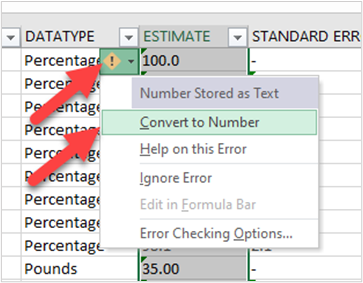
Within the ESTIMATE column (column N), are range values that include a less than (<) or greater than (>) symbol. Prior to creating a pivot table, all cells in column N will need to be converted to a numeric value (shown in the next step). Some options to consider when working with range estimates:
Remove all range values from the dataset
Remove less than or greater than symbols, but retain the range value
Assign a different numeric value that denotes estimates as range estimates (i.e., a value of 100 for all greater than ranges)
Convert estimates to numbers:
Select first data cell in the ESTIMATE column (N2).
Hold Shift+Ctrl+Down Arrow to select all estimates (column N).
Click on the exclamation point symbol at the top of the column.
Select Convert to Number.
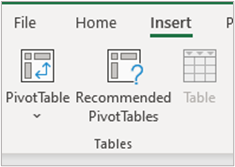
Select Insert > Pivot Table.
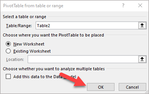
Hit OK. Note: The pivot table tool will automatically select the complete ORS dataset as your table range and create a new sheet with the table.
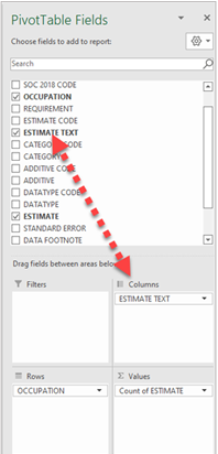
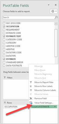
In the PivotTable Fields area, grab and drag the following fields to the following areas:
OCCUPATION -> Rows
ESTIMATE TEXT -> Columns
ESTIMATE -> Values
Note: The fields you selected and moved should all be checked.
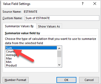
In the Values area, click the drop-down menu beside Count of ESTIMATE > Value Field Settings.
Select Sum and hit OK. Note: Sum is only a method for displaying the estimate value. No summation calculation is done.
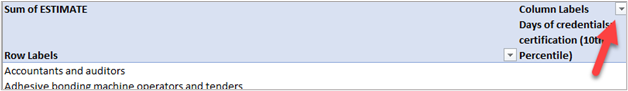
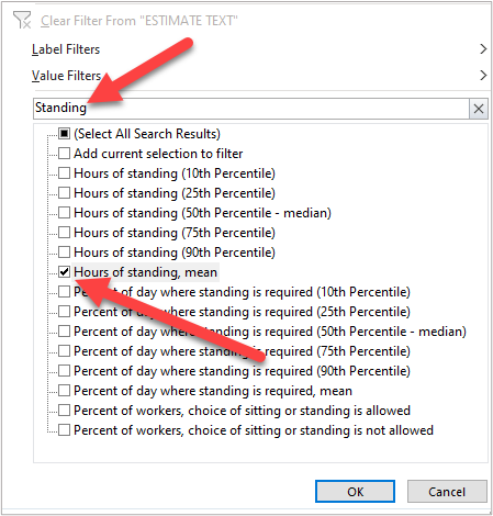
Select multiple requirements from the Columns Labels drop-down menu.
Click on the Column Labels drop-down menu arrow.
Unselect Select All.
Expand the menu to view the complete estimate text titles by hovering your cursor over the lower right-hand corner of the window until a double-headed arrow appears. Drag it and expand.
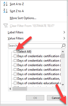
Search for the first estimate you wish to analyze by placing keywords in the text box below Value Filters. Select the estimate(s).
Check all the requirements you wish to analyze identified by the keyword search.
Click OK.
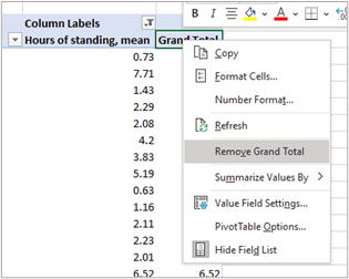
Remove the Grand Total column by selecting the Grand Total column heading cell (i.e., the cell in row 4), right click, and select Remove Grand Total from the drop-down menu.
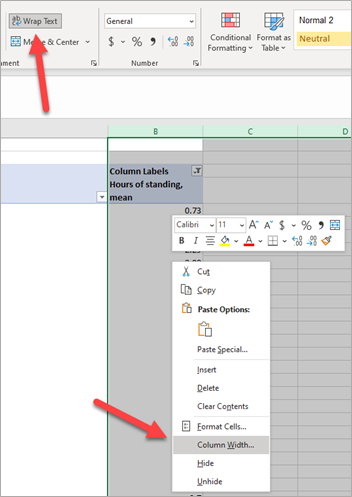
Select column B.
Hold Shift+Ctrl+Right Arrow to select the remainder columns to the right in the worksheet. All the columns should be grey indicating they are selected.
Right click somewhere in the worksheet (without selecting a cell) and select Column Width from the drop-down menu.
Enter 20 and click OK.
Click Wrap Text in the Home tab.
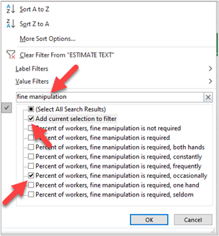
As you did above, search for additional requirements you wish to analyze using key words.
Select the additional requirements and check Add current selection to filter.
Follow the same procedure to add additional requirements.
Copy and paste as values all the data in your newly created pivot table sheet to have all data analysis tools available to analyze the data. Note: Analysis tools are limited within pivot tables.
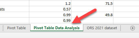
Create a new sheet to conduct your pivot table data analysis. Right click on any tab and the bottom and click Insert > Worksheet > OK.
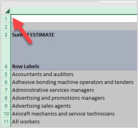
Select all the data in your pivot table sheet by clicking on the triangle in the upper left corner of your worksheet.
Hold Ctrl + C to copy the sheet to your clipboard.
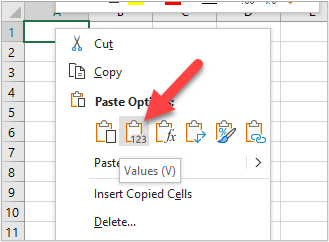
Select cell A1 in the new sheet you created to analyze your pivot table data.
Right click and select the Values (V) icon under Paste Options.
Format the new sheet.
Expand column A so that all the occupation titles are visible. To expand the width of the column, place your cursor on the border of column A, click and drag to the width desired.
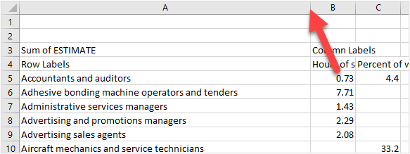
Format the remaining columns as you did in the Step above.
Delete the top 3 rows so filters can be applied to the requirement columns. The estimate text headings should be in row 1.
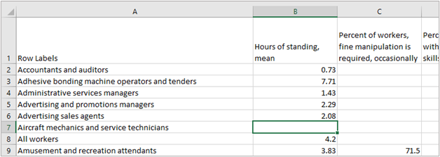
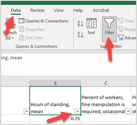
Analyze the data using the data analysis tools. Here is one example of using these tools to display only the occupations that have mean Hours of Standing equal to or less than 4 hours.
Turn on the filter tool by selecting the Filter icon in the Data tab.
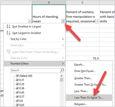
Click on arrow in the Hours of standing, mean column and select Number Filters from the drop-down menu. Then select Less Than Or Equal To.
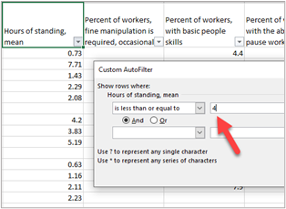
Enter 4 and select OK.
Additional resources:
Articles:
Minds at work: what’s required according to the Occupational Requirements Survey (PDF)
A look at teachers’ job requirements, employer costs, and benefits (PDF)
Occupational Requirements Survey: Third wave testing report (PDF)
Occupational Requirements Survey: results from a job observation pilot test
The Occupational Requirements Survey: estimates from preproduction testing
For additional information on occupational requirements see the ORS homepage or download the ORS complete dataset to explore the latest estimates.